使用Python从2D图像进行3D重建过程详解

2D图像的三维重建是从一组2D图像中创建对象或场景的三维模型的过程。这个技术广泛应用于计算机视觉、机器人技术和虚拟现实等领域。

在本文中，我们将解释如何使用Python执行从2D图像到三维重建的过程。我们将使用TempleRing数据集作为示例，逐步演示这个过程。该数据集包含了在对象周围的一个环上采样的阿格里真托（Agrigento）“Dioskouroi神庙”复制品的47个视图。

三维重建的关键概念

在深入了解如何使用Python从2D图像执行三维重建的详细步骤之前，让我们首先回顾一些与这个主题相关的关键概念。

深度图

深度图是一幅图像，其中每个像素代表摄像机和场景中相应点之间的距离。深度图常用于计算机视觉和机器人技术中，用于表示场景的三维结构。

有许多不同的方法可以从2D图像计算深度图，包括立体对应、结构光和飞行时间等。在本文中，我们将使用立体对应来从示例数据集计算深度图。

Point Cloud

点云是表示对象或场景形状的三维空间中的一组点。点云常用于计算机视觉和机器人技术中，用于表示场景的三维结构。

一旦我们计算出代表场景深度的深度图，我们可以使用它来计算一个三维点云。这涉及使用有关摄像机内部和外部参数的信息，将深度图中的每个像素投影回三维空间。

网格

网格是一个由顶点、边和面连接而成的表面表示。网格常用于计算机图形学和虚拟现实中，用于表示对象或场景的形状。

一旦我们计算出代表对象或场景形状的三维点云，我们可以使用它来生成一个网格。这涉及使用诸如Marching Cubes或Poisson表面重建等算法，将表面拟合到点云上。

逐步实现

现在我们已经回顾了与2D图像的三维重建相关的一些关键概念，让我们看看如何使用Python执行这个过程。我们将使用TempleRing数据集作为示例，逐步演示这个过程。下面是一个执行Temple Ring数据集中图像的三维重建的示例代码：

安装库：

pip install numpy scipy

导入库：

#importing libraries 
import cv2
import numpy as np
import matplotlib.pyplot as plt
import os

加载TempleRing数据集的图像：

# Directory containing the dataset images
dataset_dir = '/content/drive/MyDrive/templeRing'

# Initialize the list to store images
images = []# Attempt to load the grayscale images and store them in the list
for i in range(1, 48):  # Assuming images are named templeR0001.png to templeR0047.png
    img_path = os.path.join(dataset_dir, f'templeR{i:04d}.png')
    img = cv2.imread(img_path, cv2.IMREAD_GRAYSCALE)
    if img is not None:
        images.append(img)
    else:
        print(f"Warning: Unable to load 'templeR{i:04d}.png'")# Visualize the input images
num_rows = 5  # Specify the number of rows
num_cols = 10  # Specify the number of columns
fig, axs = plt.subplots(num_rows, num_cols, figsize=(15, 8))# Loop through the images and display them
for i, img in enumerate(images):
    row_index = i // num_cols  # Calculate the row index for the subplot
    col_index = i % num_cols   # Calculate the column index for the subplot
    axs[row_index, col_index].imshow(img, cmap='gray')
    axs[row_index, col_index].axis('off')# Fill any remaining empty subplots with a white background
for i in range(len(images), num_rows * num_cols):
    row_index = i // num_cols
    col_index = i % num_cols
    axs[row_index, col_index].axis('off')plt.show()

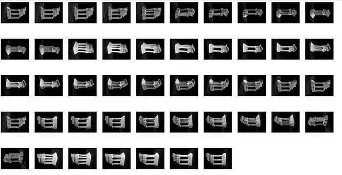
解释：这段代码加载灰度图像序列，将它们排列在网格布局中，并使用matplotlib显示它们。

为每个图像计算深度图：

# Directory containing the dataset images
dataset_dir = '/content/drive/MyDrive/templeRing'

# Initialize the list to store images
images = []# Attempt to load the grayscale images and store them in the list
for i in range(1, 48):  # Assuming images are named templeR0001.png to templeR0047.png
    img_path = os.path.join(dataset_dir, f'templeR{i:04d}.png')
    img = cv2.imread(img_path, cv2.IMREAD_GRAYSCALE)
    if img is not None:
        images.append(img)
    else:
        print(f"Warning: Unable to load 'templeR{i:04d}.png'")# Initialize the list to store depth maps
depth_maps = []# Create a StereoBM object with your preferred parameters
stereo = cv2.StereoBM_create(numDisparities=16, blockSize=15)# Loop through the images to calculate depth maps
for img in images:
    # Compute the depth map
    disparity = stereo.compute(img, img)    # Normalize the disparity map for visualization
    disparity_normalized = cv2.normalize(
        disparity, None, 0, 255, cv2.NORM_MINMAX, cv2.CV_8U)    # Append the normalized disparity map to the list of depth maps
    depth_maps.append(disparity_normalized)# Visualize all the depth maps
num_rows = 5  # Specify the number of rows
num_cols = 10  # Specify the number of columns
fig, axs = plt.subplots(num_rows, num_cols, figsize=(15, 8))for i, depth_map in enumerate(depth_maps):
    row_index = i // num_cols  # Calculate the row index for the subplot
    col_index = i % num_cols   # Calculate the column index for the subplot
    axs[row_index, col_index].imshow(depth_map, cmap='jet')
    axs[row_index, col_index].axis('off')# Fill any remaining empty subplots with a white background
for i in range(len(depth_maps), num_rows * num_cols):
    row_index = i // num_cols
    col_index = i % num_cols
    axs[row_index, col_index].axis('off')plt.show()

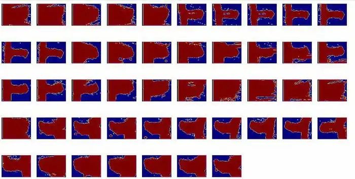
解释：这段代码负责使用Stereo Block Matching（StereoBM）算法从一系列立体图像中计算深度图。它遍历灰度立体图像列表，并为每一对相邻图像计算深度图。

可视化每个图像的深度图：

# Initialize an accumulator for the sum of depth maps
sum_depth_map = np.zeros_like(depth_maps[0], dtype=np.float64)

# Compute the sum of all depth maps
for depth_map in depth_maps:
    sum_depth_map += depth_map.astype(np.float64)
# Calculate the mean depth map by dividing the sum by the number of depth maps
mean_depth_map = (sum_depth_map / len(depth_maps)).astype(np.uint8)
# Display the mean depth map
plt.figure(figsize=(8, 6))
plt.imshow(mean_depth_map, cmap='jet')
plt.title('Mean Depth Map')
plt.axis('off')
plt.show()

输出：

解释：这段代码通过累加深度图来计算平均深度图。然后，通过将总和除以深度图的数量来计算平均值。最后，使用jet颜色图谱显示平均深度图以进行可视化。

从平均深度图计算三维点云

# Initialize an accumulator for the sum of depth maps
sum_depth_map=np.zeros_like(depth_maps[0],dtype=np.float64)

# Compute the sum of all depth maps
for depth_map in depth_maps:
    sum_depth_map += depth_map.astype(np.float64)# Calculate the mean depth map by dividing the sum by the number of depth maps
mean_depth_map = (sum_depth_map / len(depth_maps)).astype(np.uint8)# Display the mean depth map
plt.figure(figsize=(8, 6))
plt.imshow(mean_depth_map, cmap='jet')
plt.title('Mean Depth Map')
plt.axis('off')
plt.show()

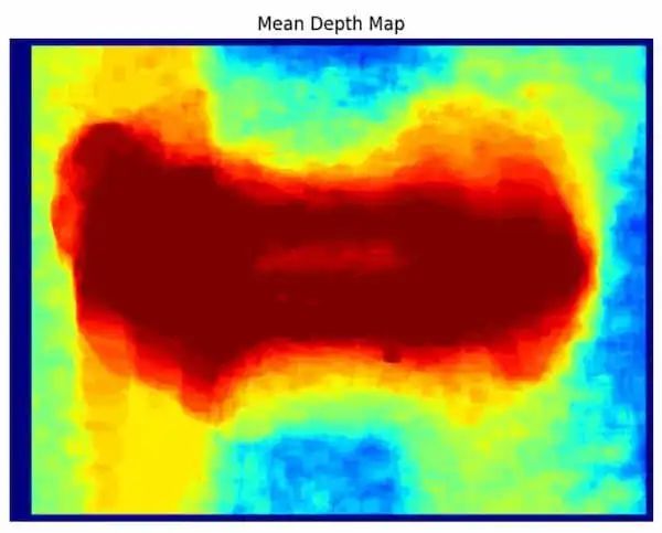
解释：这段代码通过对深度图进行累加来计算平均深度图。然后，通过将总和除以深度图的数量来计算平均值。最后，使用Jet颜色映射来可视化显示平均深度图。

计算平均深度图的三维点云

#converting into point cloud 
points_3D = cv2.reprojectImageTo3D(mean_depth_map.astype(np.float32), np.eye(4))

解释：该代码将包含点云中点的三维坐标，并且您可以使用这些坐标进行三维重建。

从点云生成网格

安装库

!pip install numpy scipy

导入库

#importing libraries 
from scipy.spatial import Delaunay
from skimage import measure
from skimage.measure import marching_cubes

生成网格

verts, faces, normals, values = measure.marching_cubes(points_3D)

解释：该代码将Marching Cubes算法应用于3D点云以生成网格。它返回定义结果3D网格的顶点、面、顶点法线和标量值。

可视化网格

fig = plt.figure()
ax = fig.add_subplot(111, projection='3d')
ax.plot_trisurf(verts[:, 0], verts[:, 1], verts[:, 2], triangles=faces)
plt.show()

输出：

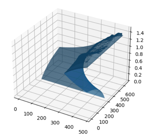
解释：该代码使用matplotlib可视化网格。它创建一个3D图并使用ax.plot_trisurf方法将网格添加到其中。

这段代码从Temple Ring数据集加载图像，并使用块匹配（block matching）进行每个图像的深度图计算，然后通过平均所有深度图来计算平均深度图，并使用它来计算每个像素的三维点云。最后，它使用Marching Cubes算法从点云生成网格并进行可视化。

结果比较

# importing the libraries
import matplotlib.pyplot as plt
from mpl_toolkits.mplot3d import Axes3D

# Create a figure with two subplots
fig, axs = plt.subplots(1, 2, figsize=(10, 5))# Visualize the original image in the first subplot
axs[0].imshow(images[0], cmap='gray')
axs[0].axis('off')
axs[0].set_title('Original')# Visualize the reconstructed mesh in the second subplot
ax = fig.add_subplot(1, 2, 2, projection='3d')
ax.plot_trisurf(verts[:, 0], verts[:, 1], verts[:, 2], triangles=faces)
ax.set_title('Reconstructed')# Show the figure
plt.show()

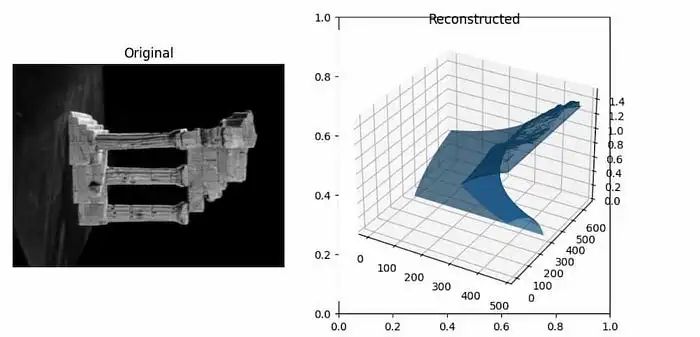
解释：在此代码中，使用matplotlib创建了包含两个子图的图形。在第一个图中，显示了来自数据集的原始图像。在第二个图中，使用3D三角形表面图可视化了重建的3D网格。

方法2

以下是执行来自TempleRing数据集图像的3D重建的另一个示例代码：

引入模块：

import cv2
import numpy as np
import matplotlib.pyplot as plt
from google.colab.patches import cv2_imshow

加载两个Temple Ring数据集图像：

# Load the PNG images (replace with your actual file paths)
image1 = cv2.imread('/content/drive/MyDrive/templeRing/templeR0001.png')
image2 = cv2.imread('/content/drive/MyDrive/templeRing/templeR0002.png'

解释：该代码使用OpenCV的cv2.imread函数从TempleRing数据集加载两个图像。

转换为灰度图：

# Convert images to grayscale
gray1 = cv2.cvtColor(image1, cv2.COLOR_BGR2GRAY)
gray2 = cv2.cvtColor(image2, cv2.COLOR_BGR2GRAY)

该代码使用OpenCV将两个图像转换为灰度图像。它们以单通道表示，其中每个像素的值表示其强度，并且没有颜色通道。

查找SIFT关键点和描述符：

# Initialize the SIFT detector
sift = cv2.SIFT_create()

# Detect keypoints and compute descriptors for both images
kp1, des1 = sift.detectAndCompute(gray1, None)
kp2, des2 = sift.detectAndCompute(gray2, None)

该代码使用尺度不变特征变换（SIFT）算法在两个图像中查找关键点和描述符。它使用OpenCV的cv2.SIFT_create()函数创建一个SIFT对象，并调用其detectAndCompute方法来计算关键点和描述符。

使用FLANN匹配器匹配描述符：

# Create a FLANN-based Matcher object
flann = cv2.FlannBasedMatcher({'algorithm': 0, 'trees': 5}, {})

# Match the descriptors using KNN (k-nearest neighbors)
matches = flann.knnMatch(des1, des2, k=2)

解释：该代码使用Fast Library for Approximate Nearest Neighbors（FLANN）匹配器对描述符进行匹配。它使用OpenCV的cv2.FlannBasedMatcher函数创建FLANN匹配器对象，并调用其knnMatch方法来找到每个描述符的k个最近邻。

使用Lowe的比率测试筛选出好的匹配项

# Apply Lowe's ratio test to select good matches
good_matches = []
for m, n in matches:
    if m.distance < 0.7 * n.distance:
        good_matches.append(m)

解释：该代码使用Lowe的比率测试筛选出好的匹配项。它使用最近邻和次近邻之间距离比的阈值来确定匹配是否良好。

提取匹配的关键点

# Extract matched keypoints
src_pts = np.float32(
    [kp1[m.queryIdx].pt for m in good_matches]).reshape(-1, 1, 2)
dst_pts = np.float32(
    [kp2[m.trainIdx].pt for m in good_matches]).reshape(-1, 1, 2)

解释：该代码从两组关键点中提取匹配的关键点，这些关键点将用于估算对齐两个图像的变换。这些关键点的坐标存储在'src_pts'和'dst_pts'中。

使用RANSAC找到单应矩阵

# Find the homography matrix using RANSAC
H, _ = cv2.findHomography(src_pts, dst_pts, cv2.RANSAC, 5.0)

在这段代码中，它使用RANSAC算法基于匹配的关键点计算描述两个图像之间的变换的单应矩阵。单应矩阵后来可以用于拉伸或变换一个图像，使其与另一个图像对齐。

使用单应矩阵将第一个图像进行变换

# Perform perspective transformation to warp image1 onto image2
height, width = image2.shape[:2]
result = cv2.warpPerspective(image1, H, (width, height))

# Display the result
cv2_imshow(result)

解释：该代码使用单应矩阵和OpenCV的cv2.warpPerspective函数将第一个图像进行变换。它指定输出图像的大小足够大，可以容纳两个图像，然后呈现结果图像。

显示原始图像和重建图像

# Display the original images and the reconstructed image side by side
fig, (ax1, ax2, ax3) = plt.subplots(1, 3, figsize=(12, 4))
ax1.imshow(cv2.cvtColor(image1, cv2.COLOR_BGR2RGB))
ax1.set_title('Image 1')
ax1.axis('off')
ax2.imshow(cv2.cvtColor(image2, cv2.COLOR_BGR2RGB))
ax2.set_title('Image 2')
ax2.axis('off')
ax3.imshow(cv2.cvtColor(result, cv2.COLOR_BGR2RGB))
ax3.set_title('Reconstructed Image')
ax3.axis('off')

plt.show()

输出：

解释：这段代码展示了在一个具有三个子图的单一图形中可视化原始图像和重建图像的过程。它使用matplotlib库显示图像，并为每个子图设置标题和轴属性。

不同的可能方法

有许多不同的方法和算法可用于从2D图像执行3D重建。选择的方法取决于诸如输入图像的质量、摄像机校准信息的可用性以及重建的期望准确性和速度等因素。

一些常见的从2D图像执行3D重建的方法包括立体对应、运动结构和多视图立体。每种方法都有其优点和缺点，对于特定应用来说，最佳方法取决于具体的要求和约束。

结论

总的来说，本文概述了使用Python从2D图像进行3D重建的过程。我们讨论了深度图、点云和网格等关键概念，并使用TempleRing数据集演示了使用两种不同方法逐步进行的过程。我们希望本文能帮助您更好地理解从2D图像进行3D重建以及如何使用Python实现这一过程。有许多可用于执行3D重建的不同方法和算法，我们鼓励您进行实验和探索，以找到最适合您需求的方法。

审核编辑：黄飞