 PyTorch教程-20.2. 深度卷积生成对抗网络

在20.1 节中,我们介绍了 GAN 工作原理背后的基本思想。我们展示了他们可以从一些简单的、易于采样的分布中抽取样本,比如均匀分布或正态分布,并将它们转换成看起来与某些数据集的分布相匹配的样本。虽然我们匹配 2D 高斯分布的示例说明了要点,但它并不是特别令人兴奋。
在本节中,我们将演示如何使用 GAN 生成逼真的图像。我们的模型将基于 Radford等人介绍的深度卷积 GAN (DCGAN)。(2015 年)。我们将借用已经证明在判别计算机视觉问题上非常成功的卷积架构,并展示如何通过 GAN 来利用它们来生成逼真的图像。
import tensorflow as tf
from d2l import tensorflow as d2l
20.2.1。口袋妖怪数据集
我们将使用的数据集是从pokemondb获得的 Pokemon 精灵的集合 。首先下载、提取和加载此数据集。
Downloading ../data/pokemon.zip from http://d2l-data.s3-accelerate.amazonaws.com/pokemon.zip...
Downloading ../data/pokemon.zip from http://d2l-data.s3-accelerate.amazonaws.com/pokemon.zip...
Downloading ../data/pokemon.zip from http://d2l-data.s3-accelerate.amazonaws.com/pokemon.zip...
Found 40597 files belonging to 721 classes.
我们将每个图像调整为64×64. 变换ToTensor 会将像素值投影到[0,1],而我们的生成器将使用 tanh 函数获取输出 [−1,1]. 因此我们用0.5意味着和0.5标准偏差以匹配值范围。
batch_size = 256
transformer = torchvision.transforms.Compose([
  torchvision.transforms.Resize((64, 64)),
  torchvision.transforms.ToTensor(),
  torchvision.transforms.Normalize(0.5, 0.5)
])
pokemon.transform = transformer
data_iter = torch.utils.data.DataLoader(
  pokemon, batch_size=batch_size,
  shuffle=True, num_workers=d2l.get_dataloader_workers())
batch_size = 256
transformer = gluon.data.vision.transforms.Compose([
  gluon.data.vision.transforms.Resize(64),
  gluon.data.vision.transforms.ToTensor(),
  gluon.data.vision.transforms.Normalize(0.5, 0.5)
])
data_iter = gluon.data.DataLoader(
  pokemon.transform_first(transformer), batch_size=batch_size,
  shuffle=True, num_workers=d2l.get_dataloader_workers())
def transform_func(X):
  X = X / 255.
  X = (X - 0.5) / (0.5)
  return X

# For TF>=2.4 use `num_parallel_calls = tf.data.AUTOTUNE`
data_iter = pokemon.map(lambda x, y: (transform_func(x), y),
            num_parallel_calls=tf.data.experimental.AUTOTUNE)
data_iter = data_iter.cache().shuffle(buffer_size=1000).prefetch(
  buffer_size=tf.data.experimental.AUTOTUNE)
WARNING:tensorflow:From /home/d2l-worker/miniconda3/envs/d2l-en-release-1/lib/python3.9/site-packages/tensorflow/python/autograph/pyct/static_analysis/liveness.py:83: Analyzer.lamba_check (from tensorflow.python.autograph.pyct.static_analysis.liveness) is deprecated and will be removed after 2023-09-23.
Instructions for updating:
Lambda fuctions will be no more assumed to be used in the statement where they are used, or at least in the same block. https://github.com/tensorflow/tensorflow/issues/56089
让我们想象一下前 20 张图像。


20.2.2。发电机
生成器需要映射噪声变量 z∈Rd, 长度-d向量,到具有宽度和高度的 RGB 图像64×64. 在 14.11 节中我们介绍了全卷积网络,它使用转置卷积层(参考 14.10 节)来扩大输入尺寸。生成器的基本块包含一个转置卷积层,然后是批量归一化和 ReLU 激活。
class G_block(nn.Module):
  def __init__(self, out_channels, in_channels=3, kernel_size=4, strides=2,
         padding=1, **kwargs):
    super(G_block, self).__init__(**kwargs)
    self.conv2d_trans = nn.ConvTranspose2d(in_channels, out_channels,
                kernel_size, strides, padding, bias=False)
    self.batch_norm = nn.BatchNorm2d(out_channels)
    self.activation = nn.ReLU()

  def forward(self, X):
    return self.activation(self.batch_norm(self.conv2d_trans(X)))
class G_block(nn.Block):
  def __init__(self, channels, kernel_size=4,
         strides=2, padding=1, **kwargs):
    super(G_block, self).__init__(**kwargs)
    self.conv2d_trans = nn.Conv2DTranspose(
      channels, kernel_size, strides, padding, use_bias=False)
    self.batch_norm = nn.BatchNorm()
    self.activation = nn.Activation('relu')

  def forward(self, X):
    return self.activation(self.batch_norm(self.conv2d_trans(X)))
class G_block(tf.keras.layers.Layer):
  def __init__(self, out_channels, kernel_size=4, strides=2, padding="same",
         **kwargs):
    super().__init__(**kwargs)
    self.conv2d_trans = tf.keras.layers.Conv2DTranspose(
      out_channels, kernel_size, strides, padding, use_bias=False)
    self.batch_norm = tf.keras.layers.BatchNormalization()
    self.activation = tf.keras.layers.ReLU()

  def call(self, X):
    return self.activation(self.batch_norm(self.conv2d_trans(X)))
默认情况下,转置卷积层使用 kh=kw=4内核,一个sh=sw=2大步前进,一个 ph=pw=1填充。输入形状为 nh′×nw′=16×16,生成器块将使输入的宽度和高度加倍。
x = torch.zeros((2, 3, 16, 16))
g_blk = G_block(20)
g_blk(x).shape
torch.Size([2, 20, 32, 32])
如果将转置卷积层更改为4×4 核心,1×1步幅和零填充。输入大小为 1×1,输出的宽度和高度将分别增加 3。
torch.Size([2, 20, 4, 4])
(2, 20, 4, 4)
生成器由四个基本块组成,将输入的宽度和高度从 1 增加到 32。同时,它首先将潜在变量投影到64×8通道,然后每次将通道减半。最后,使用转置卷积层生成输出。它进一步加倍宽度和高度以匹配所需的64×64形状,并将通道尺寸减小到 3. tanh 激活函数用于将输出值投影到(−1,1)范围。
n_G = 64
net_G = nn.Sequential(
  G_block(in_channels=100, out_channels=n_G*8,
      strides=1, padding=0),         # Output: (64 * 8, 4, 4)
  G_block(in_channels=n_G*8, out_channels=n_G*4), # Output: (64 * 4, 8, 8)
  G_block(in_channels=n_G*4, out_channels=n_G*2), # Output: (64 * 2, 16, 16)
  G_block(in_channels=n_G*2, out_channels=n_G),  # Output: (64, 32, 32)
  nn.ConvTranspose2d(in_channels=n_G, out_channels=3,
            kernel_size=4, stride=2, padding=1, bias=False),
  nn.Tanh()) # Output: (3, 64, 64)
n_G = 64
net_G = nn.Sequential()
net_G.add(G_block(n_G*8, strides=1, padding=0), # Output: (64 * 8, 4, 4)
     G_block(n_G*4), # Output: (64 * 4, 8, 8)
     G_block(n_G*2), # Output: (64 * 2, 16, 16)
     G_block(n_G),  # Output: (64, 32, 32)
     nn.Conv2DTranspose(
       3, kernel_size=4, strides=2, padding=1, use_bias=False,
       activation='tanh')) # Output: (3, 64, 64)
n_G = 64
net_G = tf.keras.Sequential([
  # Output: (4, 4, 64 * 8)
  G_block(out_channels=n_G*8, strides=1, padding="valid"),
  G_block(out_channels=n_G*4), # Output: (8, 8, 64 * 4)
  G_block(out_channels=n_G*2), # Output: (16, 16, 64 * 2)
  G_block(out_channels=n_G), # Output: (32, 32, 64)
  # Output: (64, 64, 3)
  tf.keras.layers.Conv2DTranspose(
    3, kernel_size=4, strides=2, padding="same", use_bias=False,
    activation="tanh")
])
生成一个 100 维的潜在变量来验证生成器的输出形状。
20.2.3。判别器
判别器是一个普通的卷积网络,除了它使用一个 leaky ReLU 作为它的激活函数。鉴于 α∈[0,1], 它的定义是
可以看出,如果α=0,以及一个身份函数,如果α=1. 为了α∈(0,1),leaky ReLU 是一个非线性函数,它为负输入提供非零输出。它旨在解决“垂死的 ReLU”问题,即神经元可能始终输出负值,因此无法取得任何进展,因为 ReLU 的梯度为 0。


判别器的基本块是一个卷积层,然后是一个批量归一化层和一个 leaky ReLU 激活。卷积层的超参数类似于生成器块中的转置卷积层。
class D_block(nn.Module):
  def __init__(self, out_channels, in_channels=3, kernel_size=4, strides=2,
        padding=1, alpha=0.2, **kwargs):
    super(D_block, self).__init__(**kwargs)
    self.conv2d = nn.Conv2d(in_channels, out_channels, kernel_size,
                strides, padding, bias=False)
    self.batch_norm = nn.BatchNorm2d(out_channels)
    self.activation = nn.LeakyReLU(alpha, inplace=True)

  def forward(self, X):
    return self.activation(self.batch_norm(self.conv2d(X)))
class D_block(nn.Block):
  def __init__(self, channels, kernel_size=4, strides=2,
         padding=1, alpha=0.2, **kwargs):
    super(D_block, self).__init__(**kwargs)
    self.conv2d = nn.Conv2D(
      channels, kernel_size, strides, padding, use_bias=False)
    self.batch_norm = nn.BatchNorm()
    self.activation = nn.LeakyReLU(alpha)

  def forward(self, X):
    return self.activation(self.batch_norm(self.conv2d(X)))
class D_block(tf.keras.layers.Layer):
  def __init__(self, out_channels, kernel_size=4, strides=2, padding="same",
         alpha=0.2, **kwargs):
    super().__init__(**kwargs)
    self.conv2d = tf.keras.layers.Conv2D(out_channels, kernel_size,
                       strides, padding, use_bias=False)
    self.batch_norm = tf.keras.layers.BatchNormalization()
    self.activation = tf.keras.layers.LeakyReLU(alpha)

  def call(self, X):
    return self.activation(self.batch_norm(self.conv2d(X)))
正如我们在第 7.3 节中演示的那样,具有默认设置的基本块会将输入的宽度和高度减半。例如,给定一个输入形状nh=nw=16, 具有内核形状 kh=kw=4, 步幅sh=sw=2和填充形状ph=pw=1,输出形状将是:
鉴别器是生成器的镜像。
n_D = 64
net_D = nn.Sequential(
  D_block(n_D), # Output: (64, 32, 32)
  D_block(in_channels=n_D, out_channels=n_D*2), # Output: (64 * 2, 16, 16)
  D_block(in_channels=n_D*2, out_channels=n_D*4), # Output: (64 * 4, 8, 8)
  D_block(in_channels=n_D*4, out_channels=n_D*8), # Output: (64 * 8, 4, 4)
  nn.Conv2d(in_channels=n_D*8, out_channels=1,
       kernel_size=4, bias=False)) # Output: (1, 1, 1)
n_D = 64
net_D = tf.keras.Sequential([
  D_block(n_D), # Output: (32, 32, 64)
  D_block(out_channels=n_D*2), # Output: (16, 16, 64 * 2)
  D_block(out_channels=n_D*4), # Output: (8, 8, 64 * 4)
  D_block(out_channels=n_D*8), # Outupt: (4, 4, 64 * 64)
  # Output: (1, 1, 1)
  tf.keras.layers.Conv2D(1, kernel_size=4, use_bias=False)
])
它使用带有输出通道的卷积层1作为获得单个预测值的最后一层。
20.2.4。训练
与第 20.1 节中的基本 GAN 相比,我们对生成器和鉴别器使用相同的学习率,因为它们彼此相似。此外,我们改变β1在 Adam 中(第 12.10 节)来自0.9到0.5. 它降低了动量的平滑度,即过去梯度的指数加权移动平均值,以处理快速变化的梯度,因为生成器和鉴别器相互争斗。此外,随机生成的噪声Z是一个 4-D 张量,我们正在使用 GPU 来加速计算。
def train(net_D, net_G, data_iter, num_epochs, lr, latent_dim,
     device=d2l.try_gpu()):
  loss = nn.BCEWithLogitsLoss(reduction='sum')
  for w in net_D.parameters():
    nn.init.normal_(w, 0, 0.02)
  for w in net_G.parameters():
    nn.init.normal_(w, 0, 0.02)
  net_D, net_G = net_D.to(device), net_G.to(device)
  trainer_hp = {'lr': lr, 'betas': [0.5,0.999]}
  trainer_D = torch.optim.Adam(net_D.parameters(), **trainer_hp)
  trainer_G = torch.optim.Adam(net_G.parameters(), **trainer_hp)
  animator = d2l.Animator(xlabel='epoch', ylabel='loss',
              xlim=[1, num_epochs], nrows=2, figsize=(5, 5),
              legend=['discriminator', 'generator'])
  animator.fig.subplots_adjust(hspace=0.3)
  for epoch in range(1, num_epochs + 1):
    # Train one epoch
    timer = d2l.Timer()
    metric = d2l.Accumulator(3) # loss_D, loss_G, num_examples
    for X, _ in data_iter:
      batch_size = X.shape[0]
      Z = torch.normal(0, 1, size=(batch_size, latent_dim, 1, 1))
      X, Z = X.to(device), Z.to(device)
      metric.add(d2l.update_D(X, Z, net_D, net_G, loss, trainer_D),
            d2l.update_G(Z, net_D, net_G, loss, trainer_G),
            batch_size)
    # Show generated examples
    Z = torch.normal(0, 1, size=(21, latent_dim, 1, 1), device=device)
    # Normalize the synthetic data to N(0, 1)
    fake_x = net_G(Z).permute(0, 2, 3, 1) / 2 + 0.5
    imgs = torch.cat(
      [torch.cat([
        fake_x[i * 7 + j].cpu().detach() for j in range(7)], dim=1)
       for i in range(len(fake_x)//7)], dim=0)
    animator.axes[1].cla()
    animator.axes[1].imshow(imgs)
    # Show the losses
    loss_D, loss_G = metric[0] / metric[2], metric[1] / metric[2]
    animator.add(epoch, (loss_D, loss_G))
  print(f'loss_D {loss_D:.3f}, loss_G {loss_G:.3f}, '
     f'{metric[2] / timer.stop():.1f} examples/sec on {str(device)}')
def train(net_D, net_G, data_iter, num_epochs, lr, latent_dim,
     device=d2l.try_gpu()):
  loss = gluon.loss.SigmoidBCELoss()
  net_D.initialize(init=init.Normal(0.02), force_reinit=True, ctx=device)
  net_G.initialize(init=init.Normal(0.02), force_reinit=True, ctx=device)
  trainer_hp = {'learning_rate': lr, 'beta1': 0.5}
  trainer_D = gluon.Trainer(net_D.collect_params(), 'adam', trainer_hp)
  trainer_G = gluon.Trainer(net_G.collect_params(), 'adam', trainer_hp)
  animator = d2l.Animator(xlabel='epoch', ylabel='loss',
              xlim=[1, num_epochs], nrows=2, figsize=(5, 5),
              legend=['discriminator', 'generator'])
  animator.fig.subplots_adjust(hspace=0.3)
  for epoch in range(1, num_epochs + 1):
    # Train one epoch
    timer = d2l.Timer()
    metric = d2l.Accumulator(3) # loss_D, loss_G, num_examples
    for X, _ in data_iter:
      batch_size = X.shape[0]
      Z = np.random.normal(0, 1, size=(batch_size, latent_dim, 1, 1))
      X, Z = X.as_in_ctx(device), Z.as_in_ctx(device),
      metric.add(d2l.update_D(X, Z, net_D, net_G, loss, trainer_D),
            d2l.update_G(Z, net_D, net_G, loss, trainer_G),
            batch_size)
    # Show generated examples
    Z = np.random.normal(0, 1, size=(21, latent_dim, 1, 1), ctx=device)
    # Normalize the synthetic data to N(0, 1)
    fake_x = net_G(Z).transpose(0, 2, 3, 1) / 2 + 0.5
    imgs = np.concatenate(
      [np.concatenate([fake_x[i * 7 + j] for j in range(7)], axis=1)
       for i in range(len(fake_x)//7)], axis=0)
    animator.axes[1].cla()
    animator.axes[1].imshow(imgs.asnumpy())
    # Show the losses
    loss_D, loss_G = metric[0] / metric[2], metric[1] / metric[2]
    animator.add(epoch, (loss_D, loss_G))
  print(f'loss_D {loss_D:.3f}, loss_G {loss_G:.3f}, '
     f'{metric[2] / timer.stop():.1f} examples/sec on {str(device)}')
def train(net_D, net_G, data_iter, num_epochs, lr, latent_dim,
     device=d2l.try_gpu()):
  loss = tf.keras.losses.BinaryCrossentropy(
    from_logits=True, reduction=tf.keras.losses.Reduction.SUM)

  for w in net_D.trainable_variables:
    w.assign(tf.random.normal(mean=0, stddev=0.02, shape=w.shape))
  for w in net_G.trainable_variables:
    w.assign(tf.random.normal(mean=0, stddev=0.02, shape=w.shape))

  optimizer_hp = {"lr": lr, "beta_1": 0.5, "beta_2": 0.999}
  optimizer_D = tf.keras.optimizers.Adam(**optimizer_hp)
  optimizer_G = tf.keras.optimizers.Adam(**optimizer_hp)

  animator = d2l.Animator(xlabel='epoch', ylabel='loss',
              xlim=[1, num_epochs], nrows=2, figsize=(5, 5),
              legend=['discriminator', 'generator'])
  animator.fig.subplots_adjust(hspace=0.3)

  for epoch in range(1, num_epochs + 1):
    # Train one epoch
    timer = d2l.Timer()
    metric = d2l.Accumulator(3) # loss_D, loss_G, num_examples
    for X, _ in data_iter:
      batch_size = X.shape[0]
      Z = tf.random.normal(mean=0, stddev=1,
                 shape=(batch_size, 1, 1, latent_dim))
      metric.add(d2l.update_D(X, Z, net_D, net_G, loss, optimizer_D),
            d2l.update_G(Z, net_D, net_G, loss, optimizer_G),
            batch_size)

    # Show generated examples
    Z = tf.random.normal(mean=0, stddev=1, shape=(21, 1, 1, latent_dim))
    # Normalize the synthetic data to N(0, 1)
    fake_x = net_G(Z) / 2 + 0.5
    imgs = tf.concat([tf.concat([fake_x[i * 7 + j] for j in range(7)],
                  axis=1)
             for i in range(len(fake_x) // 7)], axis=0)
    animator.axes[1].cla()
    animator.axes[1].imshow(imgs)
    # Show the losses
    loss_D, loss_G = metric[0] / metric[2], metric[1] / metric[2]
    animator.add(epoch, (loss_D, loss_G))
  print(f'loss_D {loss_D:.3f}, loss_G {loss_G:.3f}, '
     f'{metric[2] / timer.stop():.1f} examples/sec on {str(device._device_name)}')
我们用少量的 epochs 训练模型只是为了演示。为了获得更好的性能,可以将变量num_epochs设置为更大的数字。
loss_D 0.030, loss_G 7.203, 1026.4 examples/sec on cuda:0

loss_D 0.224, loss_G 6.386, 2260.7 examples/sec on gpu(0)


20.2.5。概括
-
DCGAN 架构有四个用于鉴别器的卷积层和四个用于生成器的“分数步”卷积层。
-
鉴别器是一个 4 层跨步卷积,具有批量归一化(除了它的输入层)和 leaky ReLU 激活。
-
Leaky ReLU 是一种非线性函数,可为负输入提供非零输出。它旨在解决“垂死的 ReLU”问题,并帮助梯度更容易地通过架构。
20.2.6. 练习
-
如果我们使用标准 ReLU 激活而不是 leaky ReLU 会发生什么?
-
在 Fashion-MNIST 上应用 DCGAN,看看哪个类别效果好,哪个效果不好。


 工商网监
工商网监
评论