 PyTorch教程-16.5。自然语言推理:使用注意力

我们在16.4 节介绍了自然语言推理任务和 SNLI 数据集。鉴于许多基于复杂和深层架构的模型, Parikh等人。( 2016 )提出用注意力机制解决自然语言推理,并将其称为“可分解注意力模型”。这导致模型没有循环层或卷积层,在 SNLI 数据集上以更少的参数获得了当时最好的结果。在本节中,我们将描述和实现这种用于自然语言推理的基于注意力的方法(使用 MLP),如图 16.5.1所示。

图 16.5.1本节将预训练的 GloVe 提供给基于注意力和 MLP 的架构以进行自然语言推理。
16.5.1。该模型
比保留前提和假设中标记的顺序更简单的是,我们可以将一个文本序列中的标记与另一个文本序列中的每个标记对齐,反之亦然,然后比较和聚合这些信息以预测前提和假设之间的逻辑关系。类似于机器翻译中源句和目标句之间的 token 对齐,前提和假设之间的 token 对齐可以通过注意力机制巧妙地完成。

图 16.5.2使用注意机制的自然语言推理。
图 16.5.2描述了使用注意机制的自然语言推理方法。在高层次上,它由三个联合训练的步骤组成:参与、比较和聚合。我们将在下面逐步说明它们。
import torch
from torch import nn
from torch.nn import functional as F
from d2l import torch as d2l
from mxnet import gluon, init, np, npx
from mxnet.gluon import nn
from d2l import mxnet as d2l

npx.set_np()
16.5.1.1。出席
第一步是将一个文本序列中的标记与另一个序列中的每个标记对齐。假设前提是“我确实需要睡觉”,假设是“我累了”。由于语义相似,我们可能希望将假设中的“i”与前提中的“i”对齐,并将假设中的“tired”与前提中的“sleep”对齐。同样,我们可能希望将前提中的“i”与假设中的“i”对齐,并将前提中的“需要”和“睡眠”与假设中的“疲倦”对齐。请注意,使用加权平均的这种对齐是软的,其中理想情况下较大的权重与要对齐的标记相关联。为了便于演示,图 16.5.2以硬方式显示了这种对齐方式 。
现在我们更详细地描述使用注意机制的软对齐。表示为 A=(a1,…,am)和 B=(b1,…,bn)前提和假设,其标记数为m和n,分别在哪里 ai,bj∈Rd (i=1,…,m,j=1,…,n) 是一个d维词向量。对于软对齐,我们计算注意力权重 eij∈R作为
(16.5.1)eij=f(ai)⊤f(bj),
哪里的功能f是在以下函数中定义的 MLP mlp 。的输出维度fnum_hiddens由的参数指定 mlp。
def mlp(num_inputs, num_hiddens, flatten):
  net = []
  net.append(nn.Dropout(0.2))
  net.append(nn.Linear(num_inputs, num_hiddens))
  net.append(nn.ReLU())
  if flatten:
    net.append(nn.Flatten(start_dim=1))
  net.append(nn.Dropout(0.2))
  net.append(nn.Linear(num_hiddens, num_hiddens))
  net.append(nn.ReLU())
  if flatten:
    net.append(nn.Flatten(start_dim=1))
  return nn.Sequential(*net)
def mlp(num_hiddens, flatten):
  net = nn.Sequential()
  net.add(nn.Dropout(0.2))
  net.add(nn.Dense(num_hiddens, activation='relu', flatten=flatten))
  net.add(nn.Dropout(0.2))
  net.add(nn.Dense(num_hiddens, activation='relu', flatten=flatten))
  return net
需要强调的是,在(16.5.1) f接受输入ai和bj分开而不是将它们中的一对一起作为输入。这种分解技巧只会导致m+n的应用(线性复杂度) f而不是mn应用程序(二次复杂度)。
对(16.5.1)中的注意力权重进行归一化,我们计算假设中所有标记向量的加权平均值,以获得与由索引的标记软对齐的假设表示i在前提下:
(16.5.2)βi=∑j=1nexp(eij)∑k=1nexp(eik)bj.
同样,我们为由索引的每个标记计算前提标记的软对齐j在假设中:
(16.5.3)αj=∑i=1mexp(eij)∑k=1mexp(ekj)ai.
下面我们定义Attend类来计算假设 ( beta) 与输入前提的软对齐A以及前提 ( alpha) 与输入假设的软对齐B。
class Attend(nn.Module):
  def __init__(self, num_inputs, num_hiddens, **kwargs):
    super(Attend, self).__init__(**kwargs)
    self.f = mlp(num_inputs, num_hiddens, flatten=False)

  def forward(self, A, B):
    # Shape of `A`/`B`: (`batch_size`, no. of tokens in sequence A/B,
    # `embed_size`)
    # Shape of `f_A`/`f_B`: (`batch_size`, no. of tokens in sequence A/B,
    # `num_hiddens`)
    f_A = self.f(A)
    f_B = self.f(B)
    # Shape of `e`: (`batch_size`, no. of tokens in sequence A,
    # no. of tokens in sequence B)
    e = torch.bmm(f_A, f_B.permute(0, 2, 1))
    # Shape of `beta`: (`batch_size`, no. of tokens in sequence A,
    # `embed_size`), where sequence B is softly aligned with each token
    # (axis 1 of `beta`) in sequence A
    beta = torch.bmm(F.softmax(e, dim=-1), B)
    # Shape of `alpha`: (`batch_size`, no. of tokens in sequence B,
    # `embed_size`), where sequence A is softly aligned with each token
    # (axis 1 of `alpha`) in sequence B
    alpha = torch.bmm(F.softmax(e.permute(0, 2, 1), dim=-1), A)
    return beta, alpha
class Attend(nn.Block):
  def __init__(self, num_hiddens, **kwargs):
    super(Attend, self).__init__(**kwargs)
    self.f = mlp(num_hiddens=num_hiddens, flatten=False)

  def forward(self, A, B):
    # Shape of `A`/`B`: (b`atch_size`, no. of tokens in sequence A/B,
    # `embed_size`)
    # Shape of `f_A`/`f_B`: (`batch_size`, no. of tokens in sequence A/B,
    # `num_hiddens`)
    f_A = self.f(A)
    f_B = self.f(B)
    # Shape of `e`: (`batch_size`, no. of tokens in sequence A,
    # no. of tokens in sequence B)
    e = npx.batch_dot(f_A, f_B, transpose_b=True)
    # Shape of `beta`: (`batch_size`, no. of tokens in sequence A,
    # `embed_size`), where sequence B is softly aligned with each token
    # (axis 1 of `beta`) in sequence A
    beta = npx.batch_dot(npx.softmax(e), B)
    # Shape of `alpha`: (`batch_size`, no. of tokens in sequence B,
    # `embed_size`), where sequence A is softly aligned with each token
    # (axis 1 of `alpha`) in sequence B
    alpha = npx.batch_dot(npx.softmax(e.transpose(0, 2, 1)), A)
    return beta, alpha
16.5.1.2。比较
在下一步中,我们将一个序列中的标记与与该标记软对齐的另一个序列进行比较。请注意,在软对齐中,来自一个序列的所有标记,尽管可能具有不同的注意力权重,但将与另一个序列中的标记进行比较。为了便于演示,图 16.5.2以硬方式将令牌与对齐令牌配对。例如,假设参与步骤确定前提中的“need”和“sleep”都与假设中的“tired”对齐,则将比较“tired-need sleep”对。
在比较步骤中,我们提供连接(运算符 [⋅,⋅]) 来自一个序列的标记和来自另一个序列的对齐标记到一个函数中g(一个 MLP):
(16.5.4)vA,i=g([ai,βi]),i=1,…,mvB,j=g([bj,αj]),j=1,…,n.
在(16.5.4)中,vA,i是token之间的比较i在前提和所有与 token 软对齐的假设 tokeni; 尽管 vB,j是token之间的比较j在假设和所有与标记软对齐的前提标记中j. 下面的Compare类定义了比较步骤。
class Compare(nn.Module):
  def __init__(self, num_inputs, num_hiddens, **kwargs):
    super(Compare, self).__init__(**kwargs)
    self.g = mlp(num_inputs, num_hiddens, flatten=False)

  def forward(self, A, B, beta, alpha):
    V_A = self.g(torch.cat([A, beta], dim=2))
    V_B = self.g(torch.cat([B, alpha], dim=2))
    return V_A, V_B
class Compare(nn.Block):
  def __init__(self, num_hiddens, **kwargs):
    super(Compare, self).__init__(**kwargs)
    self.g = mlp(num_hiddens=num_hiddens, flatten=False)

  def forward(self, A, B, beta, alpha):
    V_A = self.g(np.concatenate([A, beta], axis=2))
    V_B = self.g(np.concatenate([B, alpha], axis=2))
    return V_A, V_B
16.5.1.3。聚合
有两组比较向量vA,i (i=1,…,m) 和vB,j (j=1,…,n) 手头,在最后一步中,我们将汇总此类信息以推断逻辑关系。我们首先总结两组:
(16.5.5)vA=∑i=1mvA,i,vB=∑j=1nvB,j.
接下来,我们将两个汇总结果的串联提供给函数h(一个MLP)得到逻辑关系的分类结果:
(16.5.6)y^=h([vA,vB]).
聚合步骤在以下类中定义Aggregate。
class Aggregate(nn.Module):
  def __init__(self, num_inputs, num_hiddens, num_outputs, **kwargs):
    super(Aggregate, self).__init__(**kwargs)
    self.h = mlp(num_inputs, num_hiddens, flatten=True)
    self.linear = nn.Linear(num_hiddens, num_outputs)

  def forward(self, V_A, V_B):
    # Sum up both sets of comparison vectors
    V_A = V_A.sum(dim=1)
    V_B = V_B.sum(dim=1)
    # Feed the concatenation of both summarization results into an MLP
    Y_hat = self.linear(self.h(torch.cat([V_A, V_B], dim=1)))
    return Y_hat
class Aggregate(nn.Block):
  def __init__(self, num_hiddens, num_outputs, **kwargs):
    super(Aggregate, self).__init__(**kwargs)
    self.h = mlp(num_hiddens=num_hiddens, flatten=True)
    self.h.add(nn.Dense(num_outputs))

  def forward(self, V_A, V_B):
    # Sum up both sets of comparison vectors
    V_A = V_A.sum(axis=1)
    V_B = V_B.sum(axis=1)
    # Feed the concatenation of both summarization results into an MLP
    Y_hat = self.h(np.concatenate([V_A, V_B], axis=1))
    return Y_hat
16.5.1.4。把它们放在一起
通过将参与、比较和聚合步骤放在一起,我们定义了可分解的注意力模型来联合训练这三个步骤。
class DecomposableAttention(nn.Module):
  def __init__(self, vocab, embed_size, num_hiddens, num_inputs_attend=100,
         num_inputs_compare=200, num_inputs_agg=400, **kwargs):
    super(DecomposableAttention, self).__init__(**kwargs)
    self.embedding = nn.Embedding(len(vocab), embed_size)
    self.attend = Attend(num_inputs_attend, num_hiddens)
    self.compare = Compare(num_inputs_compare, num_hiddens)
    # There are 3 possible outputs: entailment, contradiction, and neutral
    self.aggregate = Aggregate(num_inputs_agg, num_hiddens, num_outputs=3)

  def forward(self, X):
    premises, hypotheses = X
    A = self.embedding(premises)
    B = self.embedding(hypotheses)
    beta, alpha = self.attend(A, B)
    V_A, V_B = self.compare(A, B, beta, alpha)
    Y_hat = self.aggregate(V_A, V_B)
    return Y_hat
class DecomposableAttention(nn.Block):
  def __init__(self, vocab, embed_size, num_hiddens, **kwargs):
    super(DecomposableAttention, self).__init__(**kwargs)
    self.embedding = nn.Embedding(len(vocab), embed_size)
    self.attend = Attend(num_hiddens)
    self.compare = Compare(num_hiddens)
    # There are 3 possible outputs: entailment, contradiction, and neutral
    self.aggregate = Aggregate(num_hiddens, 3)

  def forward(self, X):
    premises, hypotheses = X
    A = self.embedding(premises)
    B = self.embedding(hypotheses)
    beta, alpha = self.attend(A, B)
    V_A, V_B = self.compare(A, B, beta, alpha)
    Y_hat = self.aggregate(V_A, V_B)
    return Y_hat
16.5.2。训练和评估模型
现在我们将在 SNLI 数据集上训练和评估定义的可分解注意力模型。我们从读取数据集开始。
16.5.2.1。读取数据集
我们使用16.4 节中定义的函数下载并读取 SNLI 数据集 。批量大小和序列长度设置为256和50, 分别。
batch_size, num_steps = 256, 50
train_iter, test_iter, vocab = d2l.load_data_snli(batch_size, num_steps)
read 549367 examples
read 9824 examples
batch_size, num_steps = 256, 50
train_iter, test_iter, vocab = d2l.load_data_snli(batch_size, num_steps)
Downloading ../data/snli_1.0.zip from https://nlp.stanford.edu/projects/snli/snli_1.0.zip...
read 549367 examples
read 9824 examples
16.5.2.2。创建模型
我们使用预训练的 100 维 GloVe 嵌入来表示输入标记。因此,我们预先定义向量的维数 ai和bj在(16.5.1)中作为 100. 函数的输出维度f在(16.5.1) 和g在(16.5.4)中设置为 200。然后我们创建一个模型实例,初始化其参数,并加载 GloVe 嵌入以初始化输入标记的向量。
embed_size, num_hiddens, devices = 100, 200, d2l.try_all_gpus()
net = DecomposableAttention(vocab, embed_size, num_hiddens)
glove_embedding = d2l.TokenEmbedding('glove.6b.100d')
embeds = glove_embedding[vocab.idx_to_token]
net.embedding.weight.data.copy_(embeds);
embed_size, num_hiddens, devices = 100, 200, d2l.try_all_gpus()
net = DecomposableAttention(vocab, embed_size, num_hiddens)
net.initialize(init.Xavier(), ctx=devices)
glove_embedding = d2l.TokenEmbedding('glove.6b.100d')
embeds = glove_embedding[vocab.idx_to_token]
net.embedding.weight.set_data(embeds)
Downloading ../data/glove.6B.100d.zip from http://d2l-data.s3-accelerate.amazonaws.com/glove.6B.100d.zip...
16.5.2.3。训练和评估模型
与第 13.5 节split_batch中 采用单一输入(如文本序列(或图像))的 函数相反,我们定义了一个函数来采用多个输入,如小批量中的前提和假设。split_batch_multi_inputs
#@save
def split_batch_multi_inputs(X, y, devices):
  """Split multi-input `X` and `y` into multiple devices."""
  X = list(zip(*[gluon.utils.split_and_load(
    feature, devices, even_split=False) for feature in X]))
  return (X, gluon.utils.split_and_load(y, devices, even_split=False))
现在我们可以在 SNLI 数据集上训练和评估模型。
lr, num_epochs = 0.001, 4
trainer = torch.optim.Adam(net.parameters(), lr=lr)
loss = nn.CrossEntropyLoss(reduction="none")
d2l.train_ch13(net, train_iter, test_iter, loss, trainer, num_epochs, devices)
loss 0.498, train acc 0.805, test acc 0.819
14389.2 examples/sec on [device(type='cuda', index=0), device(type='cuda', index=1)]

lr, num_epochs = 0.001, 4
trainer = gluon.Trainer(net.collect_params(), 'adam', {'learning_rate': lr})
loss = gluon.loss.SoftmaxCrossEntropyLoss()
d2l.train_ch13(net, train_iter, test_iter, loss, trainer, num_epochs, devices,
        split_batch_multi_inputs)
loss 0.521, train acc 0.793, test acc 0.821
4398.4 examples/sec on [gpu(0), gpu(1)]

16.5.2.4。使用模型
最后,定义预测函数输出一对前提和假设之间的逻辑关系。
#@save
def predict_snli(net, vocab, premise, hypothesis):
  """Predict the logical relationship between the premise and hypothesis."""
  net.eval()
  premise = torch.tensor(vocab[premise], device=d2l.try_gpu())
  hypothesis = torch.tensor(vocab[hypothesis], device=d2l.try_gpu())
  label = torch.argmax(net([premise.reshape((1, -1)),
              hypothesis.reshape((1, -1))]), dim=1)
  return 'entailment' if label == 0 else 'contradiction' if label == 1
      else 'neutral'
#@save
def predict_snli(net, vocab, premise, hypothesis):
  """Predict the logical relationship between the premise and hypothesis."""
  premise = np.array(vocab[premise], ctx=d2l.try_gpu())
  hypothesis = np.array(vocab[hypothesis], ctx=d2l.try_gpu())
  label = np.argmax(net([premise.reshape((1, -1)),
              hypothesis.reshape((1, -1))]), axis=1)
  return 'entailment' if label == 0 else 'contradiction' if label == 1
      else 'neutral'
我们可以使用训练好的模型来获得样本对句子的自然语言推理结果。
predict_snli(net, vocab, ['he', 'is', 'good', '.'], ['he', 'is', 'bad', '.'])
'contradiction'
predict_snli(net, vocab, ['he', 'is', 'good', '.'], ['he', 'is', 'bad', '.'])
'contradiction'
16.5.3。概括
可分解注意力模型由三个步骤组成,用于预测前提和假设之间的逻辑关系:参与、比较和聚合。
通过注意机制,我们可以将一个文本序列中的标记与另一个文本序列中的每个标记对齐,反之亦然。这种对齐是软的,使用加权平均,理想情况下,大权重与要对齐的标记相关联。
在计算注意力权重时,分解技巧导致比二次复杂度更理想的线性复杂度。
我们可以使用预训练的词向量作为下游自然语言处理任务(如自然语言推理)的输入表示。
16.5.4。练习
使用其他超参数组合训练模型。你能在测试集上获得更好的准确性吗?
用于自然语言推理的可分解注意力模型的主要缺点是什么?
假设我们想要获得任何一对句子的语义相似度(例如,0 和 1 之间的连续值)。我们应该如何收集和标记数据集?你能设计一个带有注意力机制的模型吗?
-
自然语言
+关注
关注
1文章
292浏览量
13916 -
pytorch
+关注
关注
2文章
813浏览量
14694
发布评论请先 登录
如何开始使用PyTorch进行自然语言处理
PyTorch教程-16.7。自然语言推理:微调 BERT

注意力机制或将是未来机器学习的核心要素
一种注意力增强的自然语言推理模型aESIM


 工商网监
工商网监
评论