想化身AI领域艺术家？就使用tf.keras&Eager Execution

神经风格迁移是一项优化技术，可用于选取三幅图像，即一幅内容图像、一幅风格参考图像（例如一幅名家作品），以及您想要设定风格的输入图像，然后将它们融合在一起，这样输入图像转化后就会看起来与内容图像相似，但其呈现的是风格图像的风格。

例如，我们选取一张乌龟的图像和 Katsushika Hokusai 的《神奈川冲浪里》：

P. Lindgren 拍摄的《绿海龟》，图像来自Wikimedia Commons

如果 Hokusai 决定将他作品中海浪的纹理或风格添加到海龟图像中，这幅图看起来会是什么样？会不会是这样？

这是魔法吗？又或者只是深度学习？幸运的是，这和魔法没有任何关系：风格迁移是一项好玩又有趣的技术，可以展现神经网络的能力和内部表现形式。

神经风格迁移的原理是定义两个距离函数，一个描述两幅图像的不同之处，即 Lcontent 函数，另一个描述两幅图像的风格差异，即 Lstyle 函数。然后，给定三幅图像，一幅所需的风格图像、一幅所需的内容图像，还有一幅输入图像（用内容图像进行初始化）。我们努力转换输入图像，借助内容图像将内容距离最小化，并借助风格图像将风格距离最小化。

简而言之，我们会选取基本输入图像、我们想要匹配的内容图像以及想要匹配的风格图像。我们将使用反向传播算法最小化内容和风格距离（损失），以转换基本输入图像，创建与内容图像的内容和风格图像的风格相匹配的图像。

下文要提及的特定概念有：

在此过程中，我们会围绕下列概念积累实际经验，形成直觉认识：

Eager Execution— 使用 TensorFlow 的命令式编程环境，该环境可以立即评估操作

了解更多有关 Eager Execution 的信息

查看动态教程（许多教程都可以在Colaboratory中运行）

使用功能 API来定义模型— 我们会构建一个模型的子集，由其赋予我们使用功能 API 访问必要的中间激活的权限

利用预训练模型的特征图— 学习如何使用预训练模型及其特征图

创建自定义训练循环— 我们会研究如何设置优化器，以最小化输入参数的既定损失

我们会按照下列常规步骤来进行风格迁移：

可视化数据

对我们的数据进行基本的预处理/准备

设定损失函数

创建模型

优化损失函数

实现

首先，我们要启用Eager Execution。借助 Eager Execution，我们可以最清晰易读的方式学习这项技术

1tf.enable_eager_execution()

2print("Eager execution: {}".format(tf.executing_eagerly()))

3

4Here are the content and style images we will use:

5plt.figure(figsize=(10,10))

6

7content = load_img(content_path).astype('uint8')

8style = load_img(style_path)

9

10plt.subplot(1, 2, 1)

11imshow(content, 'Content Image')

12

13plt.subplot(1, 2, 2)

14imshow(style, 'Style Image')

15plt.show()

P. Lindgren 拍摄的《绿海龟》图，图像来自Wikimedia Commons，以及 Katsushika Hokusai 创作的《神奈川冲浪里》，图像来自公共领域

定义内容和风格表征

为了获取我们图像的内容和风格表征，我们先来看看模型内的一些中间层。中间层代表着特征图，这些特征图将随着您的深入变得越来越有序。在本例中，我们会使用 VGG19 网络架构，这是一个预训练图像分类网络。要定义我们图像的内容和风格表征，这些中间层必不可少。对于输入图像，我们会努力匹配这些中间层的相应风格和内容的目标表征。

为什么是中间层？

您可能会好奇，为什么预训练图像分类网络中的中间输出允许我们定义风格和内容表征。从较高的层面来看，我们可以通过这样的事实来解释这一现象，即网络必须要理解图像才能执行图像分类（我们的网络已接受过这样的训练）。这包括选取原始图像作为输入像素，并通过转换构建内部表征，转换就是将原始图像像素变为对图像中所呈现特征的复杂理解。这也可以部分解释卷积神经网络为何能够很好地概括图像：它们能够捕捉不同类别的不变性，并定义其中的特征（例如猫与狗），而且不受背景噪声和其他因素的影响。因此，在输入原始图像和输出类别标签之间的某个位置，模型发挥着复杂特征提取器的作用。通过访问中间层，我们可以描述输入图像的内容和风格。

具体而言，我们会从我们的网络中抽取出这些中间层：

1# Content layer where will pull our feature maps

2content_layers = ['block5_conv2']

3

4# Style layer we are interested in

5style_layers = ['block1_conv1',

6'block2_conv1',

7'block3_conv1',

8'block4_conv1',

9'block5_conv1'

10]

11

12num_content_layers = len(content_layers)

13num_style_layers = len(style_layers)

模型

在本例中，我们将加载VGG19，并将输入张量输入模型中。这样，我们就可以提取内容图像、风格图像和所生成图像的特征图（随后提取内容和风格表征）。

依照论文中的建议，我们使用 VGG19 模型。此外，由于 VGG19 是一个较为简单的模型（与 ResNet、Inception 等模型相比），其特征图实际更适用于风格迁移。

为了访问与我们的风格和内容特征图相对应的中间层，我们需要使用 Keras功能 API来获取相应的输出，从而使用所需的输出激活定义我们的模型。

借助功能 API，定义模型时仅需定义输入和输出即可：model = Model(inputs, outputs)。

1def get_model():

2""" Creates our model with access to intermediate layers.

3

4This function will load the VGG19 model and access the intermediate layers.

5These layers will then be used to create a new model that will take input image

6and return the outputs from these intermediate layers from the VGG model.

7Returns:

8returns a keras model that takes image inputs and outputs the style and

9content intermediate layers.

10"""

11# Load our model. We load pretrained VGG, trained on imagenet data (weights=’imagenet’)

12vgg = tf.keras.applications.vgg19.VGG19(include_top=False, weights='imagenet')

13vgg.trainable = False

14# Get output layers corresponding to style and content layers

15style_outputs = [vgg.get_layer(name).output for name in style_layers]

16content_outputs = [vgg.get_layer(name).output 17for name in content_layers]

18model_outputs = style_outputs + content_outputs

19# Build model

20return models.Model(vgg.input, model_outputs)

在上图的代码片段中，我们将加载预训练图像分类网络。然后，我们会抓取此前定义的兴趣层。之后，我们将定义一个模型，将模型的输入设置为图像，将输出设置为风格层和内容层的输出。换言之，我们创建的模型将接受输入图像并输出内容和风格中间层！

定义和创建我们的损失函数（内容和风格距离）

内容损失：

我们的内容损失定义实际上相当简单。我们将向网络传递所需的内容图像和基本输入图像，这样，我们的模型会返回中间层输出（自上文定义的层）。然后，我们只需选取这些图像的两个中间表征之间的欧氏距离。

更正式地讲，内容损失是一个函数，用于描述内容与我们的输入图像 x 和内容图像 p 之间的距离。设 Cₙₙ 为预训练深度卷积神经网络。再次强调，我们在本例中使用VGG19。设 X 为任意图像，则 Cₙₙ(x) 为 X 馈送的网络。用 Fˡᵢⱼ(x)∈ Cₙₙ(x) 和 Pˡᵢⱼ(x) ∈ Cₙₙ(x) 分别描述网络在 l 层上输入为 x 和 p 的中间层表征。之后，我们可以将内容距离（损失）正式描述为：

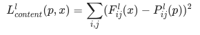
我们以常规方式执行反向传播算法，以便将内容损失降至最低。这样，我们可以更改初始图像，直至其在某个层（在 content_layer 中定义）中生成与原始内容图像相似的响应。

该操作非常容易实现。同样地，在我们的输入图像 x 和内容图像 p 馈送的网络中，其会将 L 层的输入特征图视为输入图像，然后返回内容距离。

1def get_content_loss(base_content, target):

2return tf.reduce_mean(tf.square(base_content - target))

风格损失：

计算风格损失时涉及的内容较多，但遵循相同的原则，这次我们要为网络提供基本输入图像和风格图像。但我们要比较的是这两个输出的格拉姆矩阵，而非基本输入图像和风格图像的原始中间输出。

在数学上，我们将基本输入图像 x 和风格图像 a 的风格损失描述为这些图像的风格表征（格拉姆矩阵）之间的距离。我们将图像的风格表征描述为由格拉姆矩阵 Gˡ 给定的不同过滤响应间的相关关系，其中 Gˡᵢⱼ 为 l 层中矢量化特征图 i 和 j 之间的内积。我们可以看到，针对特定图像的特征图生成的 Gˡᵢⱼ 表示特征图 i 和 j 之间的相关关系。

要为我们的基本输入图像生成风格，我们需要对内容图像执行梯度下降法，将其转换为与原始图像的风格表征匹配的图像。我们通过最小化风格图像与输入图像的特征相关图之间的均方距离来进行此项操作。每层对总风格损失的贡献用以下公式描述

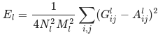
其中 Gˡᵢⱼ 和 Aˡᵢⱼ 分别为输入图像 x 和风格图像 a 在 l 层的风格表征。Nl 表示特征图的数量，每个图的大小为 Ml= 高度 ∗ 宽度。因此，每层的总风格损失为

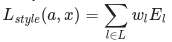
其中，我们用系数 wl 来衡量每层损失的贡献。在这个例子中，我们平均地衡量每个层：

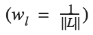
这实施起来很简单：

1def gram_matrix(input_tensor):

2# We make the image channels first

3channels = int(input_tensor.shape[-1])

4a = tf.reshape(input_tensor, [-1, channels])

5n = tf.shape(a)[0]

6gram = tf.matmul(a, a, transpose_a=True)

7return gram / tf.cast(n, tf.float32)

8

9def get_style_loss(base_style, gram_target):

10"""Expects two images of dimension h, w, c"""

11# height, width, num filters of each layer

12height, width, channels = base_style.get_shape().as_list()

13gram_style = gram_matrix(base_style)

14return tf.reduce_mean(tf.square(gram_style - 15gram_target))

运行梯度下降法

如果您对梯度下降法/反向传播算法不熟悉，或需要复习一下，那您一定要查看此资源。

在本例中，我们使用Adam优化器来最小化我们的损失。我们迭代更新输出图像，以最大限度地减少损失：我们不是更新与网络有关的权重，而是训练我们的输入图像以使损失最小化。为此，我们必须知道如何计算损失和梯度。请注意，我们推荐使用 L-BFGS 优化器（如果您熟悉此算法的话），但本教程并未使用该优化器，因为本教程旨在阐述使用 Eager Execution 的最佳实践。通过使用 Adam，我们可以借助自定义训练循环来说明 autograd/梯度带的功能。

计算损失和梯度

我们会定义一些辅助函数，这些函数会加载我们的内容和风格图像，通过网络将它们向前馈送，然后从我们的模型输出内容和风格的特点表征。

1def get_feature_representations(model, content_path, style_path):

2"""Helper function to compute our content and style feature representations.

3

4This function will simply load and preprocess both the content and style

5images from their path. Then it will feed them through the network to obtain

6the outputs of the intermediate layers.

7

8Arguments:

9 model: The model that we are using.

10content_path: The path to the content image. 11style_path: The path to the style image

12

13Returns:

14returns the style features and the content features.

15"""

16# Load our images in

17content_image = load_and_process_img(content_path)

18style_image = load_and_process_img(style_path)

19

20# batch compute content and style features

21stack_images = np.concatenate([style_image, content_image], axis=0)

22model_outputs = model(stack_images)

23# Get the style and content feature representations from our model

24

25 style_features = [style_layer[0] for style_layer in model_outputs[:num_style_layers]]

26content_features = [content_layer[1] for content_layer in model_outputs[num_style_layers:]]

27return style_features, content_features

这里我们使用tf.GradientTape来计算梯度。这样，我们可以通过追踪操作来利用可用的自动微分，以便之后计算梯度。它会记录正向传递期间的操作，并能够计算关于向后传递的输入图像的损失函数梯度。

1def compute_loss(model, loss_weights, init_image, gram_style_features, content_features):

2"""This function will compute the loss total loss.

3

4 Arguments:

5model: The model that will give us access to the intermediate layers

6loss_weights: The weights of each contribution of each loss function.

7(style weight, content weight, and total variation weight)

8init_image: Our initial base image. This image is what we are updating with

9 our optimization process. We apply the gradients wrt the loss we are

10 calculating to this image.

11 gram_style_features: Precomputed gram matrices corresponding to the

12 defined style layers of interest.

13 content_features: Precomputed outputs from defined content layers of

14 interest.

15

16Returns:

17returns the total loss, style loss, content loss, and total variational loss

18"""

19style_weight, content_weight, total_variation_weight = loss_weights

20

21# Feed our init image through our model. This will give us the content and

22# style representations at our desired layers. Since we're using eager

23# our model is callable just like any other function!

24model_outputs = model(init_image)

25

26style_output_features = model_outputs[:num_style_layers]

27content_output_features = model_outputs[num_style_layers:]

28

29style_score = 0

30content_score = 0

31

32# Accumulate style losses from all layers

33# Here, we equally weight each contribution of each loss layer

34weight_per_style_layer = 1.0 / float(num_style_layers)

35for target_style, comb_style in zip(gram_style_features, style_output_features):

36style_score += weight_per_style_layer * get_style_loss(comb_style[0], target_style)

37

38# Accumulate content losses from all layers

39weight_per_content_layer = 1.0 / float(num_content_layers)

40for target_content, comb_content in zip(content_features, content_output_features):

41content_score += weight_per_content_layer* get_content_loss(comb_content[0], target_content)

42

43style_score *= style_weight

44content_score *= content_weight

45total_variation_score = total_variation_weight * total_variation_loss(init_image)

46

47# Get total loss

48loss = style_score + content_score + total_variation_score

49return loss, style_score, content_score, total_variation_score

然后计算梯度就很简单了：

1def compute_grads(cfg):

2with tf.GradientTape() as tape:

3all_loss = compute_loss(**cfg)

4# Compute gradients wrt input image

5total_loss = all_loss[0]

6return tape.gradient(total_loss, cfg['init_image']), all_loss

应用并运行风格迁移流程

要实际进行风格迁移：

1def run_style_transfer(content_path,

2style_path,

3num_iterations=1000,

4content_weight=1e3,

5style_weight = 1e-2):

6display_num = 100

7# We don't need to (or want to) train any layers of our model, so we set their trainability

8# to false.

9model = get_model()

10for layer in model.layers:

11layer.trainable = False

12

13# Get the style and content feature representations (from our specified intermediate layers)

14style_features, content_features = get_feature_representations(model, content_path, style_path)

15gram_style_features = [gram_matrix(style_feature) for style_feature in style_features]

16

17# Set initial image

18init_image = load_and_process_img(content_path)

19init_image = tfe.Variable(init_image, dtype=tf.float32)

20# Create our optimizer

21opt = tf.train.AdamOptimizer(learning_rate=10.0)

22

23# For displaying intermediate images

24iter_count = 1

25

26# Store our best result

27best_loss, best_img = float('inf'), None

28

29# Create a nice config

30loss_weights = (style_weight, content_weight)

31cfg = {

32'model': model,

33'loss_weights': loss_weights,

34'init_image': init_image,

35'gram_style_features': gram_style_features,

36'content_features': content_features

37}

38

39# For displaying

40plt.figure(figsize=(15, 15))

41num_rows = (num_iterations / display_num) // 5

42start_time = time.time()

43global_start = time.time()

44

45norm_means = np.array([103.939, 116.779, 123.68])

46min_vals = -norm_means

47max_vals = 255 - norm_means

48for i in range(num_iterations):

49grads, all_loss = compute_grads(cfg)

50loss, style_score, content_score = all_loss

51# grads, _ = tf.clip_by_global_norm(grads, 5.0)

52opt.apply_gradients([(grads, init_image)])

53clipped = tf.clip_by_value(init_image, min_vals, max_vals)

54init_image.assign(clipped)

55end_time = time.time()

56

57if loss < best_loss:    

58# Update best loss and best image from total loss.

59 best_loss = loss

60best_img = init_image.numpy()

61

62if i % display_num == 0:

63print('Iteration: {}'.format(i))

64print('Total loss: {:.4e}, '

65'style loss: {:.4e}, '

66'content loss: {:.4e}, '

67'time: {:.4f}s'.format(loss, style_score, content_score, time.time() - start_time))

68start_time = time.time()

69

70# Display intermediate images

71if iter_count > num_rows * 5: continue

72plt.subplot(num_rows, 5, iter_count)

73# Use the .numpy() method to get the concrete numpy array

74plot_img = init_image.numpy()

75plot_img = deprocess_img(plot_img)

76plt.imshow(plot_img)

77plt.title('Iteration {}'.format(i + 1))

78

79iter_count += 1

80print('Total time: {:.4f}s'.format(time.time() - global_start))

81

82return best_img, best_loss

就是这样！

我们在海龟图像和 Hokusai 的《神奈川冲浪里》上运行该流程：

1best, best_loss = run_style_transfer(content_path,

2style_path,

3verbose=True,

4show_intermediates=True)

P.Lindgren 拍摄的《绿海龟》图[CC BY-SA 3.0 (https://creativecommons.org/licenses/by-sa/3.0)]，图片来自 Wikimedia Common

观察这一迭代过程随时间发生的变化：

下面有一些关于神经风格迁移用途的很棒示例。快来看看吧！

图宾根的图像 — 拍摄者：Andreas Praefcke [GFDL (http://www.gnu.org/copyleft/fdl.html) 或 CC BY 3.0 (https://creativecommons.org/licenses/by/3.0)]，图像来自Wikimedia Commons；以及梵高的《星月夜》，图像来自公共领域

图宾根的图像 — 拍摄者：Andreas Praefcke [GFDL (http://www.gnu.org/copyleft/fdl.html) 或 CC BY 3.0 (https://creativecommons.org/licenses/by/3.0)]，图片来自Wikimedia Commons，和 Vassily Kandinsky 所作的《构图 7》，图片来自公共领域