OpenCV中的直线拟合

直线拟合原理

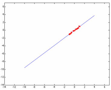
给出多个点，然后根据这些点拟合出一条直线，这个最常见的算法是多约束方程的最小二乘拟合，如下图所示:

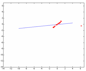
但是当这些点当中有一个或者几个离群点(outlier)时候，最小二乘拟合出来的直线就直接翻车成这样了：

原因是最小二乘无法在估算拟合的时候剔除或者降低离群点的影响，于是一个聪明的家伙出现了，提出了基于权重的最小二乘拟合估算方法，这样就避免了翻车。根据高斯分布，离群点权重应该尽可能的小，这样就可以降低它的影响，OpenCV中的直线拟合就是就权重最小二乘完成的，在生成权重时候OpenCV支持几种不同的距离计算方法，分别如下：

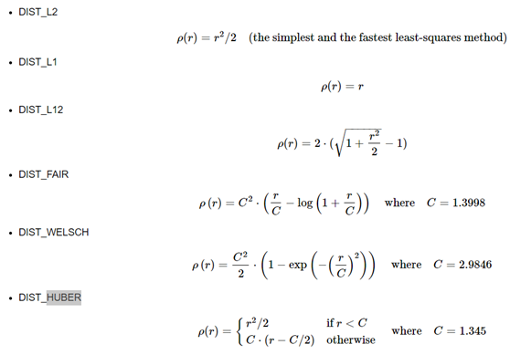
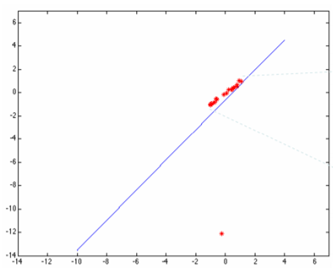
其中DIST_L2是最原始的最小二乘，最容易翻车的一种拟合方式，虽然速度快点。然后用基于权重的最小二乘估算拟合结果如下：

函数与实现源码分析

OpenCV中直线拟合函数支持上述六种距离计算方式，函数与参数解释如下：

void cv::fitLine(         InputArray    points,         OutputArray   line,         int   distType,         double    param,         double    reps,         double    aeps)

points是输入点集合

line是输出的拟合参数，支持2D与3D

distType是选择距离计算方式

param 是某些距离计算时生成权重需要的参数

reps 是前后两次原点到直线的距离差值，可以看成拟合精度高低

aeps是前后两次角度差值，表示的是拟合精度

六种权重的计算更新实现如下：

staticvoidweightL1(float*d,intcount,float*w)
{
inti;


for(i=0;i< count; i++ )
    {
        double t = fabs( (double) d[i] );
        w[i] = (float)(1. / MAX(t, eps));
    }
}


static void weightL12( float *d, int count, float *w )
{
    int i;


    for( i = 0; i < count; i++ )
    {
        w[i] = 1.0f / (float) std::sqrt( 1 + (double) (d[i] * d[i] * 0.5) );
    }
}




static void weightHuber( float *d, int count, float *w, float _c )
{
    int i;
    const float c = _c <= 0 ? 1.345f : _c;


    for( i = 0; i < count; i++ )
    {
        if( d[i] < c )
            w[i] = 1.0f;
        else
            w[i] = c/d[i];
    }
}




static void weightFair( float *d, int count, float *w, float _c )
{
    int i;
    const float c = _c == 0 ? 1 / 1.3998f : 1 / _c;


    for( i = 0; i < count; i++ )
    {
        w[i] = 1 / (1 + d[i] * c);
    }
}


static void weightWelsch( float *d, int count, float *w, float _c )
{
    int i;
    const float c = _c == 0 ? 1 / 2.9846f : 1 / _c;


    for( i = 0; i < count; i++ )
    {
        w[i] = (float) std::exp( -d[i] * d[i] * c * c );
    }
}

拟合计算的代码实现：

staticvoidfitLine2D_wods(constPoint2f*points,intcount,float*weights,float*line)
{
CV_Assert(count>0);
doublex=0,y=0,x2=0,y2=0,xy=0,w=0;
doubledx2,dy2,dxy;
inti;
floatt;

//Calculatingtheaverageofxandy...
if(weights==0)
{
for(i=0;i< count; i += 1 )
        {
            x += points[i].x;
            y += points[i].y;
            x2 += points[i].x * points[i].x;
            y2 += points[i].y * points[i].y;
            xy += points[i].x * points[i].y;
        }
        w = (float) count;
    }
    else
    {
        for( i = 0; i < count; i += 1 )
        {
            x += weights[i] * points[i].x;
            y += weights[i] * points[i].y;
            x2 += weights[i] * points[i].x * points[i].x;
            y2 += weights[i] * points[i].y * points[i].y;
            xy += weights[i] * points[i].x * points[i].y;
            w += weights[i];
        }
    }

    x /= w;
    y /= w;
    x2 /= w;
    y2 /= w;
    xy /= w;

    dx2 = x2 - x * x;
    dy2 = y2 - y * y;
    dxy = xy - x * y;

    t = (float) atan2( 2 * dxy, dx2 - dy2 ) / 2;
    line[0] = (float) cos( t );
    line[1] = (float) sin( t );

    line[2] = (float) x;
    line[3] = (float) y;
}

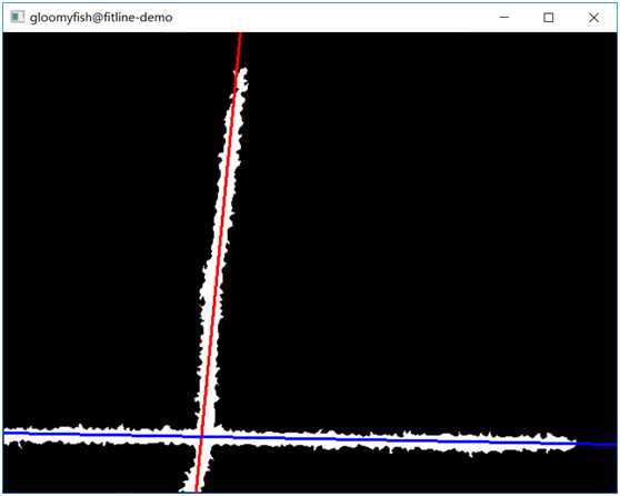
案例：直线拟合

有如下的原图：

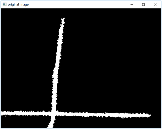
通过OpenCV的距离变换，骨架提取，然后再直线拟合，使用DIST_L1得到的结果如下：

审核编辑：彭静