神经网络超参数调优

神经网络在通信行业和研究中的使用十分常见，但令人遗憾的是，大部分应用都未能产出足以运行其他算法的高性能网络。

应用数学家在开发新型优化算法时，喜欢进行功能测试，有时也被称为人造景观。人造景观有助于从以下方面比较各算法的性能：

· 收敛（算出答案的速度）

· 精准度（与正确答案的接近程度）

· 稳健性（是否所有功能表现优良，或仅一小部分如此）

· 综合表现（如概念复杂度）

浏览有关功能优化测试的维基词条，就会发现有些功能很难对付。很多功能因找出优化算法的问题而被广泛使用。但本文将讨论一项看似微不足道的功能——Beale功能。

Beale功能

Beale功能如下图所示：

Beale功能是测试功能的原因在于，它能在坡度极小的平坦区域内评估调优算法的性能。在这种情况下，基于坡度的优化算法程序难以有效地学习，因此很难达到最小值。

本文接下来将按照GitHub库里的Jupyter笔记本教程开展讨论，以得出解决人造景观的可行方式。该景观类似于神经网络的损失平面。训练神经网络的目的是通过某种形式的优化找到损失平面上的最小值——典型的随机坡度减少。

在学习使用高难度的优化功能后，本文读者能充分应对施行神经网络时遇到的实际问题场景。

测试神经网络前，首先需要给功能下定义能并找出最小值（否则无法确定为正确答案）。第一步（引进相关软件包后），在笔记本中定义Beale功能：

# define Beale‘s function which we want to minimize

def objective（X）：

x = X［0］; y = X［1］

return （1.5 - x + x*y）**2 + （2.25 - x + x*y**2）**2 + （2.625 - x + x*y**3）**2

已知此案例中（由我们构想）最小值的大概范围及栅极网孔的步长，第二步设置功能边界值。

# function boundaries

xmin， xmax， xstep = -4.5， 4.5， .9

ymin， ymax， ystep = -4.5， 4.5， .9

根据以上信息制作一组点状网孔栅极，就可以找出最小值。

# Let’s create some points

x1， y1 = np.meshgrid（np.arange（xmin， xmax + xstep， xstep）， np.arange（ymin， ymax + ystep， ystep））

现在，得出（非常）初步的结论。

# initial guess

x0 = ［4.， 4.］

f0 = objective（x0）

print （f0）

然后使用scipy.optimize功能，得出答案。

bnds = （（xmin， xmax）， （ymin， ymax））

minimum = minimize（objective， x0， bounds=bnds）

print（minimum）

答案结果如下：

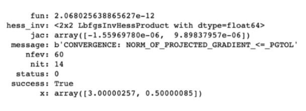
答案似乎是（3，0.5）。如果把这些值填入等式，这确实是最小值（维基上也显示如此）。

接下来进入神经网络部分。

神经网络的优化

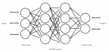
神经网络可以被定义为一个结合输入并猜测输出的系统。幸运的话，在得出被称作“地面实况”的结果后，将之与神经网络的各种输出进行比对，就能计算错误。因此，神经网络首先进行猜测，然后计算错误功能；再次猜测，将错误最小化；再次猜测，直到错误最小化。这就是优化。

神经网络中最常使用的优化算法是GD（gradient descent，坡降）类型。坡降中使用的客观功能正是想缩至最小的损失功能。

本教程的重头戏是Keras，因此再回顾一下。

Keras复习

Keras是一个深度学习Python库，可同时在Theano和TensorFlow上运行，它们也是两个强大的快速数字计算Python库，分别在脸书和谷歌上创建发布。

Keras旨在开发尽可能快捷简单的深度学习模型，以运用在研究和实用程序中。Keras使用Python 2.7或3.5语言运行，可无缝切换至GPU和CPU运行。

Keras基于一个模型的概念。在其核心有一些按顺序线性排列的层级，称为顺序模型。Keras还提供功能性界面，可定义复杂模型，如多产出模型、定向非循环图以及有共有层级的模型。

可使用顺序模型总结Keras的深度学习模型构建，如下所示：

1. 定义模型：创建顺序模型，增加层级。

2. 编译模型：具体设置损失功能和优化器，调用the .compile（）功能。

3. 调试模型：调用the .fit（） 功能用数据测试模型。

4. 进行预测：通过调用.evaluate（） 和.predict（）功能，使用该模型对新数据生成新预测。

有些人可能会疑惑——如何在运行模型过程中检测其性能？这是个好问题，答案就是使用回叫。

回叫：训练模型过程中进行监测

通过使用回叫，可在训练的任何阶段监测模型。回叫是指对训练程序中特定阶段使用的一系列功能。使用回叫，可在训练过程中观察模型内部状态及数据。可向顺序或模型分类的the .fit（）方法传输一系列回叫（作为关键词变元回叫）。回叫的相关方法将会在训练的每一个阶段使用。

· 大众所熟悉的Keras回叫功能是keras.callbacks.History（）。这是.fit（）方法自带的。

· keras.callbacks.ModelCheckpoint也很有用，可在训练中存储特定阶段模型的重量。如果模型长时间运行且出现系统故障，该功能会很有效果。使用该功能后任何数据都不会遗失。比如，只有当累加器计算且观测到改进时，存储模型重量才是适宜的做法。

· 可监测的大批错误停止改进时，keras.callbacks.EarlyStopping功能停止训练。

· keras.callbacks.LearningRateScheduler功能将改变训练过程中的学习速度。

之后将应用一些回叫。

首先需要引进很多不同的功能，以方便操作。

import tensorflow as tf

import keras

from keras import layers

from keras import models

from keras import utils

from keras.layers import Dense

from keras.models import Sequential

from keras.layers import Flatten

from keras.layers import Dropout

from keras.layers import Activation

from keras.regularizers import l2

from keras.optimizers import SGD

from keras.optimizers import RMSprop

from keras import datasets

from keras.callbacks import LearningRateScheduler

from keras.callbacks import History

from keras import losses

from sklearn.utils import shuffle

print（tf.VERSION）

print（tf.keras.__version__）

如果想要网络使用随机数字但结果可重复，还可以执行的一个步骤是使用随机种子。随机种子每次产出同样顺序的数字，哪怕它们是伪随机的（有助于比较模型和测试可复制性）。

# fix random seed for reproducibility

np.random.seed（5）

第一步——确定网络拓扑（不一定是优化，但也至关重要）

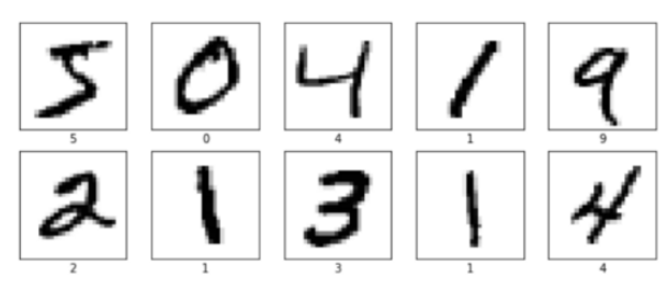
这一步将使用MNIST数据集，其包含手写数字（0到9）的灰度图，28×28像素维度。每个像素是8位数，因此其数值范围在0到255之间。

Keras有此内置功能，因此能便捷地获取数据集。

mnist = keras.datasets.mnist

（x_train， y_train），（x_test， y_test） = mnist.load_data（）

x_train.shape， y_train.shape

X和Y数据的产出分别是（60000， 28， 28）和（60000，1）。建议打印一些数据，检验数值（同时需要数据类型）。

可通过观察每个数字的图像来检查训练数据，以确保数据中没有任何遗漏的。

plt.figure（figsize=（10，10））

for i in range（10）：

plt.subplot（5，5，i+1）

plt.xticks（［］）

plt.yticks（［］）

plt.grid（False）

plt.imshow（x_train［i］， cmap=plt.cm.binary）

plt.xlabel（y_train［i］）

最后一项检查是针对训练维度和测试集，这一步骤操作相对简单：

print（f‘We have {x_train.shape［0］} train samples’）

print（f‘We have {x_test.shape［0］} test samples’）

有60，000个训练图像和10，000个测试图像。之后要预处理数据。

预处理数据

运行神经网络前，需要预处理数据（以下步骤可任意替换顺序）：

· 首先，需要将2D图像阵列转为1D（扁平化）。可使用numpy.reshape（）功能进行阵列重塑，或使用Keras的方法：keras.layers.Flatten层级，可将2D阵列（28×28像素）图像转化为1D阵列图像（28 * 28 = 784像素）。

· 然后需要将像素值调至正常状态（将数值调整为0到1之间），转换如下：

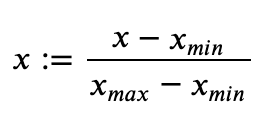
在案例中，最小值为0，最大值为255，因此公式为：：=/255。

# normalize the data

x_train， x_test = x_train / 255.0， x_test / 255.0

# reshape the data into 1D vectors

x_train = x_train.reshape（60000， 784）

x_test = x_test.reshape（10000， 784）

num_classes = 10

# Check the column length

x_train.shape［1］

现在数据中需要一个独热码。

# Convert class vectors to binary class matrices

y_train = keras.utils.to_categorical（y_train， num_classes）

y_test = keras.utils.to_categorical（y_test， num_classes）

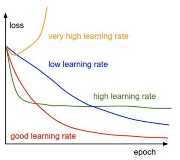
第二步——调整学习速度

最常用的优化算法之一是随机坡降（SGD）。其中可调优的超参数是学习速度，动量，衰变和nesterov项。

学习速度在每批结束时控制重量，并且动量控制先前重量如何影响当前重量。衰变表示每次更新时学习速度的下降幅度。nesterov取值“True”或“False”取决于是否要应用Nesterov动量。

这些超参数的通常数值是lr = 0.01，衰变= 1e-6，动量= 0.9，nesterov = True。

学习速度超参数会存在于优化功能中，如下所示。 Keras在SGDoptimizer中具有默认学习速度调度器，会通过随机坡降的优化算法降低学习速度。 学习速度随着以下公式降低：

lr=lr×1/（1+decayepoch）

接下来在Keras中实施学习速度适应时间表。 先从SGD开始，学习速度数值为0.1。 然后针对模型训练60个时期并将衰变参数设置为0.0016（0.1 / 60）。其中还包括动量值0.8，因为它在使用、适应学习速度时运作良好。

pochs=60

learning_rate = 0.1

decay_rate = learning_rate / epochs

momentum = 0.8

sgd = SGD（lr=learning_rate， momentum=momentum， decay=decay_rate， nesterov=False）

接下来开始构建神经网络：

# build the model

input_dim = x_train.shape［1］

lr_model = Sequential（）

lr_model.add（Dense（64， activation=tf.nn.relu， kernel_initializer=‘uniform’，

input_dim = input_dim））

lr_model.add（Dropout（0.1））

lr_model.add（Dense（64， kernel_initializer=‘uniform’， activation=tf.nn.relu））

lr_model.add（Dense（num_classes， kernel_initializer=‘uniform’， activation=tf.nn.softmax））

# compile the model

lr_model.compile（loss=‘categorical_crossentropy’，

optimizer=sgd，

metrics=［‘acc’］）

现在可以运行模型，看看它的表现如何。机器花费了大约20分钟，各人的机器运行速度不一。

%%time

# Fit the model

batch_size = int（input_dim/100）

lr_model_history = lr_model.fit（x_train， y_train，

batch_size=batch_size，

epochs=epochs，

verbose=1，

validation_data=（x_test， y_test））

运行完毕后，可以把准确度和损失功能绘制为训练和测试集的时期函数，以查看网络运行情况。

# Plot the loss function

fig， ax = plt.subplots（1， 1， figsize=（10，6））

ax.plot（np.sqrt（lr_model_history.history［‘loss’］）， ‘r’， label=‘train’）

ax.plot（np.sqrt（lr_model_history.history［‘val_loss’］）， ‘b’ ，label=‘val’）

ax.set_xlabel（r‘Epoch’， fontsize=20）

ax.set_ylabel（r‘Loss’， fontsize=20）

ax.legend（）

ax.tick_params（labelsize=20）

# Plot the accuracy

fig， ax = plt.subplots（1， 1， figsize=（10，6））

ax.plot（np.sqrt（lr_model_history.history［‘acc’］）， ‘r’， label=‘train’）

ax.plot（np.sqrt（lr_model_history.history［‘val_acc’］）， ‘b’ ，label=‘val’）

ax.set_xlabel（r‘Epoch’， fontsize=20）

ax.set_ylabel（r‘Accuracy’， fontsize=20）

ax.legend（）

ax.tick_params（labelsize=20）

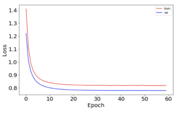
损失函数图如下：

准确度如下：

现在应用自定义学习速度。

使用LearningRateScheduler改变自定义学习速度

编写一个执行指数学习速度衰变的函数，如下公式所示：

=0×^（ - ）

这与之前非常相似，因此会在一个代码块中执行此操作，并描述差异。

# solution

epochs = 60

learning_rate = 0.1 # initial learning rate

decay_rate = 0.1

momentum = 0.8

# define the optimizer function

sgd = SGD（lr=learning_rate， momentum=momentum， decay=decay_rate， nesterov=False）

input_dim = x_train.shape［1］

num_classes = 10

batch_size = 196

# build the model

exponential_decay_model = Sequential（）

exponential_decay_model.add（Dense（64， activation=tf.nn.relu， kernel_initializer=‘uniform’， input_dim = input_dim））

exponential_decay_model.add（Dropout（0.1））

exponential_decay_model.add（Dense（64， kernel_initializer=‘uniform’， activation=tf.nn.relu））

exponential_decay_model.add（Dense（num_classes， kernel_initializer=‘uniform’， activation=tf.nn.softmax））

# compile the model

exponential_decay_model.compile（loss=‘categorical_crossentropy’，

optimizer=sgd，

metrics=［‘acc’］）

# define the learning rate change

def exp_decay（epoch）：

lrate = learning_rate * np.exp（-decay_rate*epoch）

return lrate

# learning schedule callback

loss_history = History（）

lr_rate = LearningRateScheduler（exp_decay）

callbacks_list = ［loss_history， lr_rate］

# you invoke the LearningRateScheduler during the .fit（） phase

exponential_decay_model_history = exponential_decay_model.fit（x_train， y_train，

batch_size=batch_size，

epochs=epochs，

callbacks=callbacks_list，

verbose=1，

validation_data=（x_test， y_test））

此处看到，唯一改变的是被定义的exp_decay函数，以及它在LearningRateScheduler函数中的使用。注意本次还选择向模型添加一些回叫。

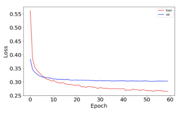
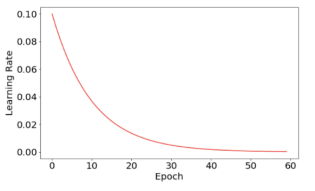
现在可以将学习速度和损失功能绘制为时期数量的函数。学习速度图非常平稳，因为它符合预定义的指数衰变函数。

与之前相比，损失函数更为平稳。

这表明开发学习速度调度程序有助于提高神经网络的性能。

第三步——选择优化器和损失函数

在构建模型并使用它进行预测时，如为图像（“猫”，“平面”等）加标签，希望通过定义“损失”函数来衡量成败（或目标函数）。优化目标是有效计算使该损失函数最小化的参数/权重。Keras提供各种类型的损失函数。

有时“损失”函数可以测量“距离”，通过符合问题或数据集的各种方式在两个数据点之间定义这个“距离”。使用的距离取决于数据类型和正在处理的特定问题。例如，在自然语言处理（分析文本数据）中，汉明距离的使用更为常见。

距离

· 欧几里德（Euclidean）

· 曼哈顿（Manhattan）

· 如汉明等距离用于测量弦之间的距离。 “carolin”和“cathrin”之间的汉明距离为3。

损失函数

· MSE（用于回归）

· 分类交叉熵（用于分类）

· 二元交叉熵（用于分类）

# build the model

input_dim = x_train.shape［1］

model = Sequential（）

model.add（Dense（64， activation=tf.nn.relu， kernel_initializer=‘uniform’，

input_dim = input_dim）） # fully-connected layer with 64 hidden units

model.add（Dropout（0.1））

model.add（Dense（64， kernel_initializer=‘uniform’， activation=tf.nn.relu））

model.add（Dense（num_classes， kernel_initializer=‘uniform’， activation=tf.nn.softmax））

# defining the parameters for RMSprop （I used the keras defaults here）

rms = RMSprop（lr=0.001， rho=0.9， epsilon=None， decay=0.0）

model.compile（loss=‘categorical_crossentropy’，

optimizer=rms，

metrics=［‘acc’］）

第4步——确定批量大小和时期数量

批量大小定义通过网络传播的样本数。

例如，有1000个训练样本，并且要设置batch_size为100。算法从训练数据集中获取前100个样本（从第1到第100个）训练网络。接下来，需要另外100个样本（从第101到第200）并再次训练网络。此过程需一直执行直至传播完样本。

使用批量大小的优点《所有样本数量的优点：

· 所需内存更小。由于使用较少样本训练网络，整体训练过程需要较小的内存。如果无法将整个数据集放入机器的内存中，那么这一点尤为重要。

· 通常，使用小批量的网络培训得更快，原因是每次传播后会更新权重。

使用批量大小的缺点《所有样本的数量的缺点：

· 批次越小，梯度的估计就越不准确。

时期数是一个超参数，定义学习算法在整个训练数据集中的工作次数。

一个时期意味着训练数据集中的每个样本都有机会更新内部模型参数。时期由一个或多个批次组成。

选择批量大小或时期数没有硬性和快速的规则，并且增加时期数不一定比较少时期数产生更好的结果。

%%time

batch_size = input_dim

epochs = 60

model_history = model.fit（x_train， y_train，

batch_size=batch_size，

epochs=epochs，

verbose=1，

validation_data=（x_test， y_test））

score = model.evaluate（x_test， y_test， verbose=0）print（‘Test loss：’， score［0］）print（‘Test accuracy：’， score［1］）

fig， ax = plt.subplots（1， 1， figsize=（10，6））ax.plot（np.sqrt（model_history.history［‘acc’］）， ‘r’， label=‘train_acc’）ax.plot（np.sqrt（model_history.history［‘val_acc’］）， ‘b’ ，label=‘val_acc’）ax.set_xlabel（r‘Epoch’， fontsize=20）ax.set_ylabel（r‘Accuracy’， fontsize=20）ax.legend（）ax.tick_params（labelsize=20）

fig， ax = plt.subplots（1， 1， figsize=（10，6））ax.plot（np.sqrt（model_history.history［‘loss’］）， ‘r’， label=‘train’）ax.plot（np.sqrt（model_history.history［‘val_loss’］）， ‘b’ ，label=‘val’）ax.set_xlabel（r‘Epoch’， fontsize=20）ax.set_ylabel（r‘Loss’， fontsize=20）ax.legend（）ax.tick_params（labelsize=20）

第5步——随机重启

此方法似乎无法Keras中实现，但可以通过更改keras.callbacks.LearningRateScheduler轻松完成。本文将此作为练习留给读者，它主要是在有限时期数之后重置学习速度。

使用交叉验证调整超参数

现在无需手动尝试不同值，而可使用Scikit-Learn的GridSearchCV，为超参数尝试几个值，并比较结果。

为使用Keras进行交叉验证，将运用到Scikit-Learn API的包装器。其将Sequential Keras模型使用（仅单输入）作为Scikit-Learn工作流程的一部分。

以下为两个包装器：

keras.wrappers.scikit_learn.KerasClassifier（build_fn = None，** sk_params），它实现了Scikit-Learn分类器接口。

keras.wrappers.scikit_learn.KerasRegressor（build_fn = None，** sk_params），它实现了Scikit-Learn回归量接口。

import numpy

from sklearn.model_selection import GridSearchCV

from keras.wrappers.scikit_learn import KerasClassifier

尝试不同的权重初始化

将尝试通过交叉验证进行优化的第一个超参数是不同的权重初始化。

# let‘s create a function that creates the model （required for KerasClassifier）

# while accepting the hyperparameters we want to tune

# we also pass some default values such as optimizer=’rmsprop‘

def create_model（init_mode=’uniform‘）：

# define model

model = Sequential（）

model.add（Dense（64， kernel_initializer=init_mode， activation=tf.nn.relu， input_dim=784））

model.add（Dropout（0.1））

model.add（Dense（64， kernel_initializer=init_mode， activation=tf.nn.relu））

model.add（Dense（10， kernel_initializer=init_mode， activation=tf.nn.softmax））

# compile model

model.compile（loss=’categorical_crossentropy‘，

optimizer=RMSprop（），

metrics=［’accuracy‘］）

return model

%%time

seed = 7

numpy.random.seed（seed）

batch_size = 128

epochs = 10

model_CV = KerasClassifier（build_fn=create_model， epochs=epochs，

batch_size=batch_size， verbose=1）

# define the grid search parameters

init_mode = ［’uniform‘， ’lecun_uniform‘， ’normal‘， ’zero‘，

’glorot_normal‘， ’glorot_uniform‘， ’he_normal‘， ’he_uniform‘］

param_grid = dict（init_mode=init_mode）

grid = GridSearchCV（estimator=model_CV， param_grid=param_grid， n_jobs=-1， cv=3）

grid_result = grid.fit（x_train， y_train）

# print results

print（f’Best Accuracy for {grid_result.best_score_} using {grid_result.best_params_}‘）

means = grid_result.cv_results_［’mean_test_score‘］

stds = grid_result.cv_results_［’std_test_score‘］

params = grid_result.cv_results_［’params‘］

for mean， stdev， param in zip（means， stds， params）：

print（f’ mean={mean：.4}， std={stdev：.4} using {param}‘）

GridSearch结果如下：

可以看到，从使用lecun_uniform初始化或glorot_uniform初始化的模型中得出最好的结果，并且可以获得近97％的准确度。

将神经网络模型保存为JSON

分层数据格式（HDF5）用于存储大阵列数据，包括神经网络中权重的值。

可以安装HDF5 Python模块：pip install h5py

Keras有助于使用JSON格式描述和保存任何模型。

from keras.models import model_from_json

# serialize model to JSON

model_json = model.to_json（）

with open（“model.json”， “w”） as json_file：

json_file.write（model_json）

# save weights to HDF5

model.save_weights（“model.h5”）

print（“Model saved”）

# when you want to retrieve the model： load json and create model

json_file = open（’model.json‘， ’r‘）

saved_model = json_file.read（）

# close the file as good practice

json_file.close（）

model_from_json = model_from_json（saved_model）

# load weights into new model

model_from_json.load_weights（“model.h5”）

print（“Model loaded”）

使用多个超参数进行交叉验证

通常人们对一个参数变化的方式不感兴趣，而对多个参数变化如何影响结果感到好奇。可以同时对多个参数进行交叉验证，尝试它们的组合。

注意：神经网络中的交叉验证需要大量计算。在实验之前要三思！将需要验证的要素数量相乘，查看有多少组合。使用k折交叉验证评估每个组合（k是我们选择的参数）。

例如，可以选择搜索不同的值：

· 批量大小

· 时期数量

· 初始化模式

选项被指定到字典中并传递给GridSearchCV。

现在对批量大小、时期数和初始化程序组合执行GridSearch。

# repeat some of the initial values here so we make sure they were not changed

input_dim = x_train.shape［1］

num_classes = 10

# let’s create a function that creates the model （required for KerasClassifier）

# while accepting the hyperparameters we want to tune

# we also pass some default values such as optimizer=‘rmsprop’

def create_model_2（optimizer=‘rmsprop’， init=‘glorot_uniform’）：

model = Sequential（）

model.add（Dense（64， input_dim=input_dim， kernel_initializer=init， activation=‘relu’））

model.add（Dropout（0.1））

model.add（Dense（64， kernel_initializer=init， activation=tf.nn.relu））

model.add（Dense（num_classes， kernel_initializer=init， activation=tf.nn.softmax））

# compile model

model.compile（loss=‘categorical_crossentropy’，

optimizer=optimizer，

metrics=［‘accuracy’］）

return model

%%time

# fix random seed for reproducibility （this might work or might not work

# depending on each library‘s implenentation）

seed = 7

numpy.random.seed（seed）

# create the sklearn model for the network

model_init_batch_epoch_CV = KerasClassifier（build_fn=create_model_2， verbose=1）

# we choose the initializers that came at the top in our previous cross-validation！！

init_mode = ［’glorot_uniform‘， ’uniform‘］

batches = ［128， 512］

epochs = ［10， 20］

# grid search for initializer， batch size and number of epochs

param_grid = dict（epochs=epochs， batch_size=batches， init=init_mode）

grid = GridSearchCV（estimator=model_init_batch_epoch_CV，

param_grid=param_grid，

cv=3）

grid_result = grid.fit（x_train， y_train）

# print results

print（f’Best Accuracy for {grid_result.best_score_：.4} using {grid_result.best_params_}‘）

means = grid_result.cv_results_［’mean_test_score‘］

stds = grid_result.cv_results_［’std_test_score‘］

params = grid_result.cv_results_［’params‘］

for mean， stdev， param in zip（means， stds， params）：

print（f’mean={mean：.4}， std={stdev：.4} using {param}‘）

最后一个问题：如果在GridSearchCV中必须循环的参数数量和值的数量特别大，该怎么办？

这可能是一个棘手的问题。想象一下，有5个参数以及为每个参数选择的10个可能值。可能组合的数量是10，这意味着必须训练一个庞大的网络。显然，这种操作会很疯狂，所以通常使用RandomizedCV。

RandomizedCV允许人们指定所有可能的参数。对于交叉验证中的每个折叠，它选择用于当前模型的随机参数子集。最后，用户可以选择最佳参数集并将其用作近似解。