Ultra96皮肤癌AI构建

描述

我们为什么要构建皮肤癌 AI？

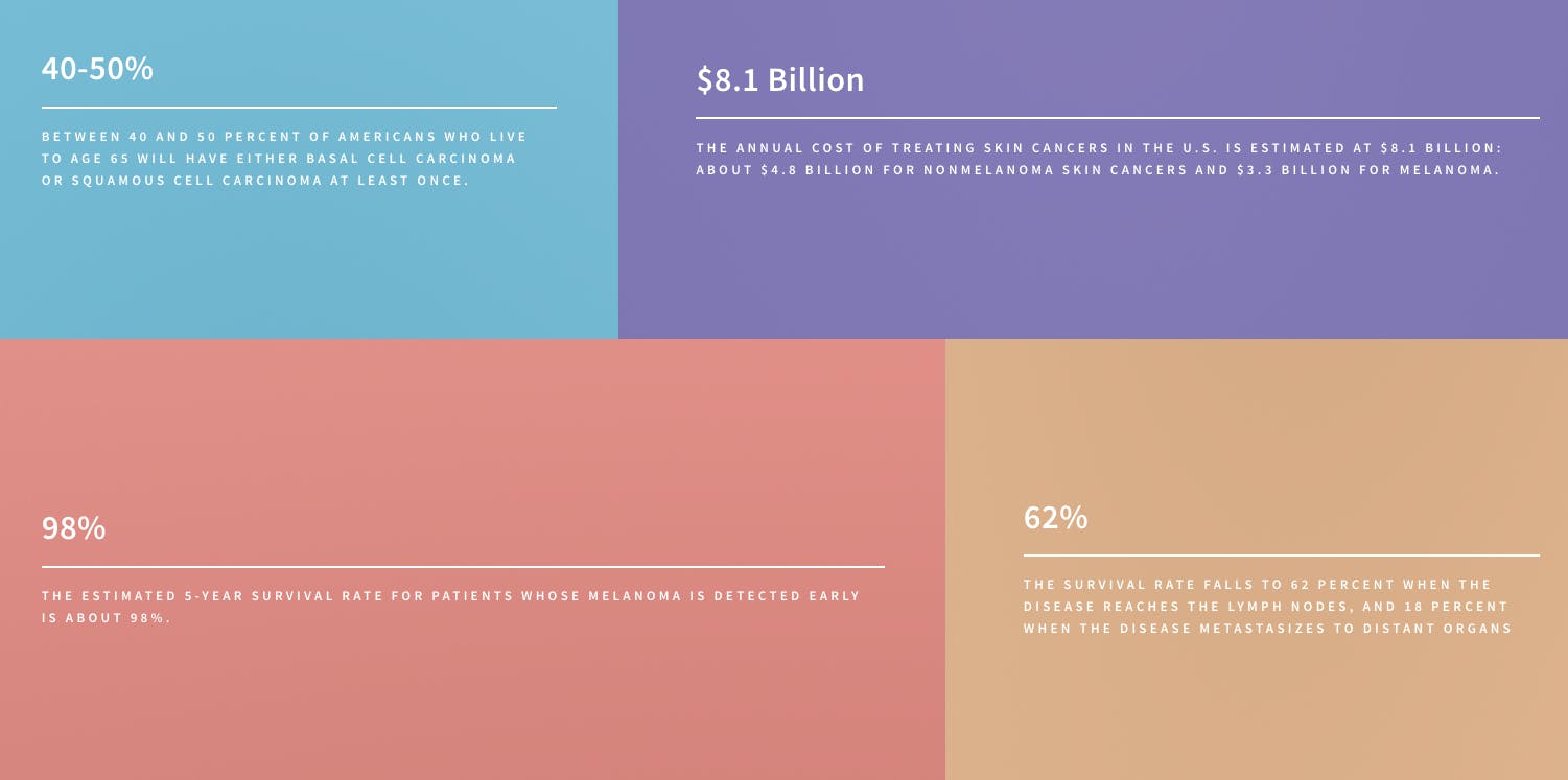
根据皮肤癌基金会的数据，美国一半的人口在 65 岁之前被诊断出患有某种形式的皮肤癌。早期发现的存活率几乎是 98%，但当癌症到达淋巴结时，存活率会下降到 62%转移到远处器官时为 18%。借助皮肤癌 AI，我们希望利用人工智能的力量提供尽可能广泛的早期检测。

什么是人工智能以及如何使用它？

深度学习最近是机器学习的一大趋势，最近的成功为构建这样的项目铺平了道路。在这个示例中，我们将特别关注计算机视觉和图像分类。为此，我们将使用深度学习算法、卷积神经网络 (CNN) 通过 Caffe 框架构建痣、黑色素瘤和脂溢性角化病图像分类器。

在本文中，我们将重点关注监督学习，它需要在服务器上进行训练以及在边缘部署。我们的目标是构建一个可以实时检测癌症图像的机器学习算法，这样您就可以构建自己的基于人工智能的皮肤癌分类设备。

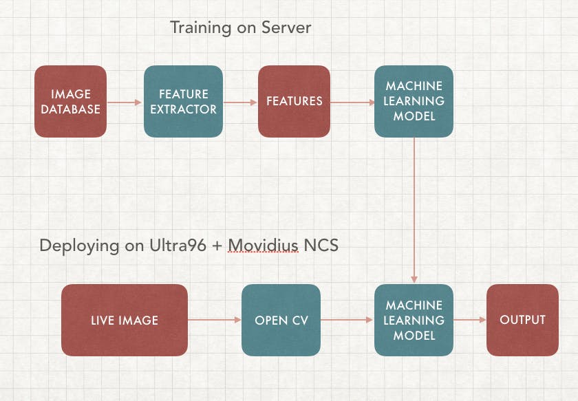
我们的应用程序将包括两部分，第一部分是训练，我们将使用不同的癌症图像数据库集来训练具有相应标签的机器学习算法（模型）。第二部分是在边缘部署，它使用我们训练过的相同模型并在边缘设备上运行，在本例中是通过 Ultra96 FPGA 的 Movidius 神经计算棒。这样 VPU 可以运行推理，而 FPGA 可以执行 OpenCV

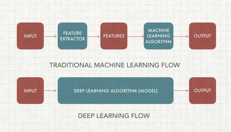
传统机器学习 (ML) 与深度学习

这可能是人工智能中被问得最多的问题，一旦你学会了如何去做，它就相当简单了。为了理解这一点，我们首先必须了解机器学习图像分类的工作原理。

机器学习需要特征提取和模型训练。我们首先必须使用领域知识来提取可用于我们的 ML 算法模型的特征，一些例子包括SIFT和HoG。之后，我们可以使用包含所有图像特征和标签的数据集来训练我们的机器学习模型。

传统 ML 和深度学习之间的主要区别在于特征工程。传统 ML 使用手动编程的功能，而深度学习会自动执行。特征工程相对困难，因为它需要领域专业知识并且非常耗时。深度学习不需要特征工程，可以更准确

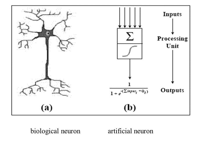
人工神经网络 (ANN)

根据技术百科，“人工神经元网络（ANN）是一种基于生物神经网络结构和功能的计算模型。” 人工神经元网络在技术上模拟人类生物神经元的工作方式，它具有有限数量的输入、与它们相关的权重和激活功能。节点的激活函数定义了给定输入或一组输入的该节点的输出，编码复杂是非线性的。数据的模式。当输入进来时，激活函数应用到输入的权重和以生成输出。人工神经元相互连接形成一个网络，因此称为人工神经元网络（ANN）。

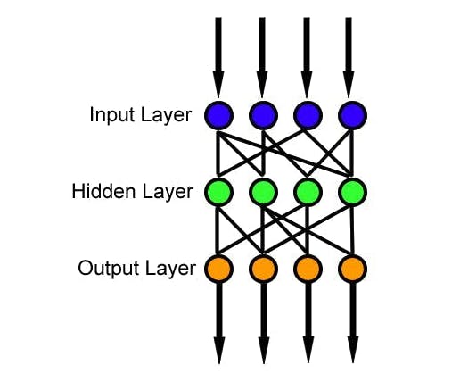
前馈神经网络是一种人工神经网络，其中节点之间的连接不形成循环，这是最简单的人工神经网络形式。它有 3 层，输入层、隐藏层和输出层，其中数据通过输入层进入，通过隐藏层到达输出节点，如下图所示。我们可以有多个隐藏层，模型的复杂度与隐藏层的大小相关。

训练数据和损失函数是用于训练神经网络的两个元素。训练数据由图像和相应的标签组成；损失函数是衡量分类过程中不准确的函数。一旦获得了这两个元素，我们就使用反向传播算法和梯度下降来训练 ANN。

卷积神经网络 (CNN)

卷积神经网络是一类深度前馈人工神经网络，最常用于分析视觉图像，因为它旨在模拟动物视觉皮层上的生物行为。它由卷积层和池化层组成，因此网络可以对图像属性进行编码。

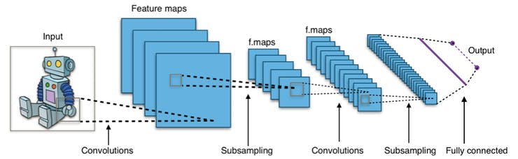
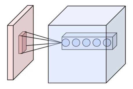
卷积层的参数由一组具有小感受野的可学习过滤器（或内核）组成。这样，图像可以在空间上进行卷积，计算过滤器条目和输入之间的点积，并生成该过滤器的二维激活图。通过这种方式，网络可以学习在检测到输入图像空间特征上的特殊特征时可以激活的过滤器。

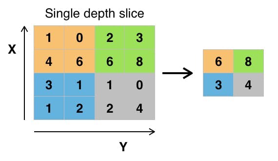
池化层是非线性下采样的一种形式。它将输入图像划分为一组不重叠的矩形，并为每个这样的子区域输出最大值。其思想是不断减小输入表示的空间大小以减少网络中的参数量和计算量，因此它也可以控制过拟合。最大池化是最常见的非线性池化类型。根据维基百科，“池化通常与大小为 2x2 的过滤器一起应用，每个深度切片的步长为 2。大小为 2x2 且步长为 2 的池化层将输入图像缩小到其原始大小的 1/4。”

皮肤癌 AI 组件

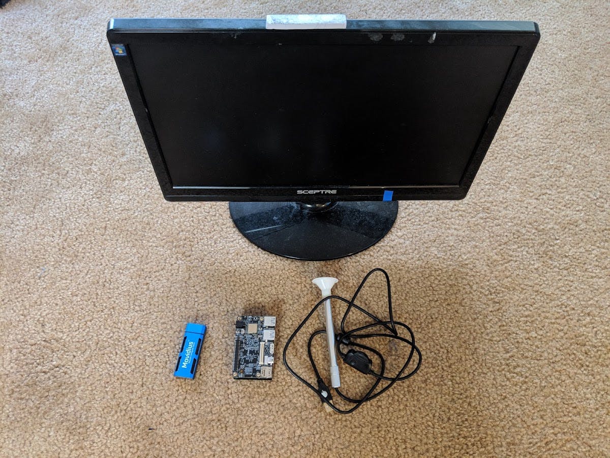
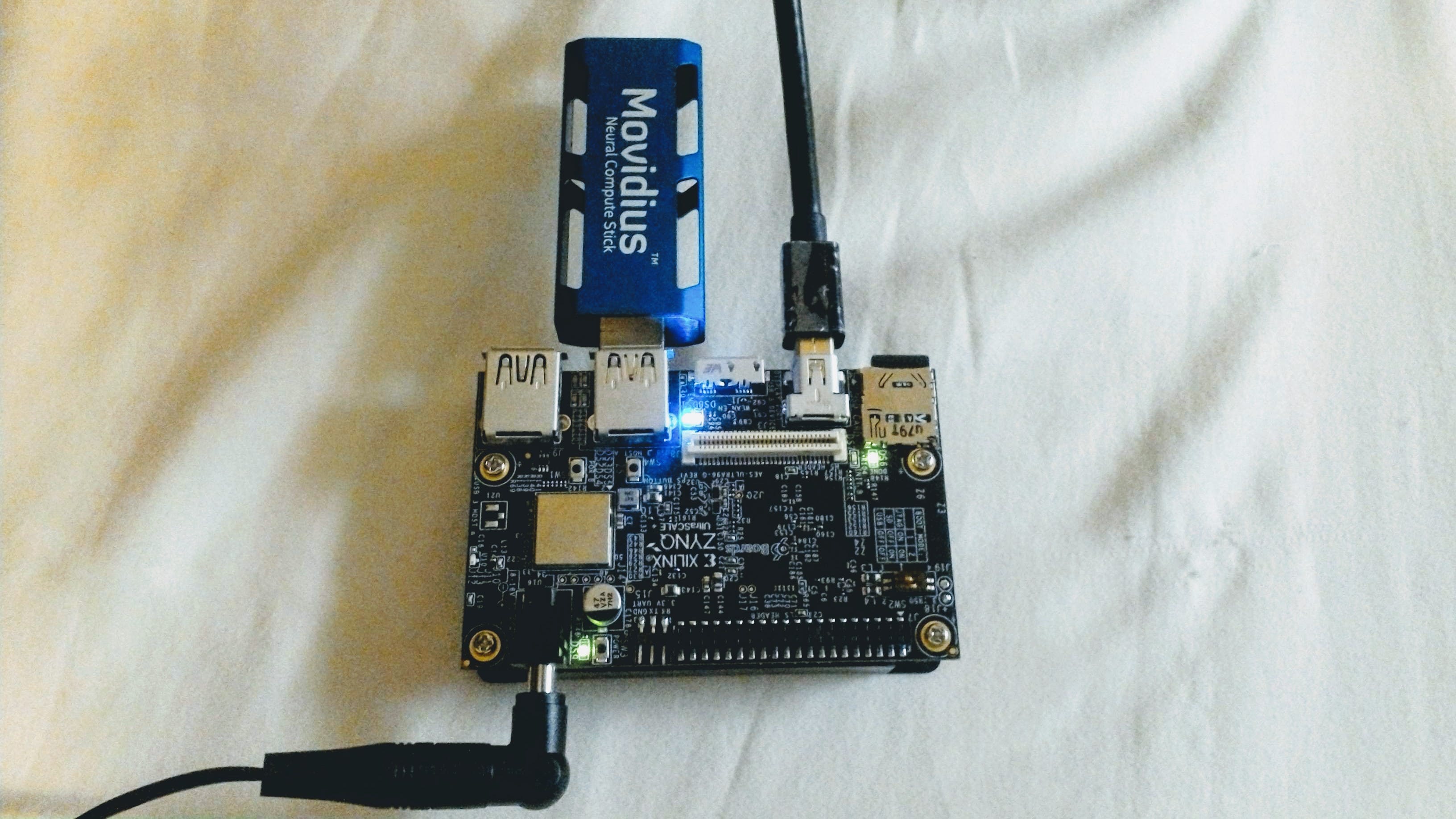
该项目所需的设备非常简单，您可以使用计算机和 USB Movidius 神经计算棒和 Ultra96 板来完成。

• Ultra96 板
• 内窥镜相机
• Movidius 神经计算棒
• 屏幕或监视器

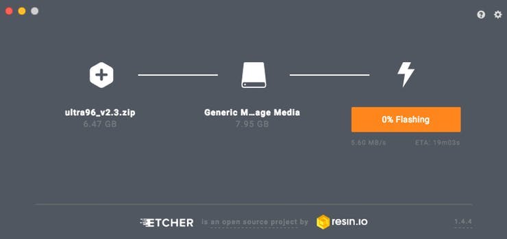
第 1 步：安装 PYNQ Linux

Ultra96 是相当新的，但支持小组非常友好地让基本的 Ubuntu 运行，这很重要，因为这让我可以在 ultra96 上构建不同的平台。编译好的debian可以从https://fileserver.linaro.org/owncloud/index.php/s/jTt3MYSuwtLuf9d下载，之后我们可以使用ether之类的工具把它加载到mini-sd卡上。

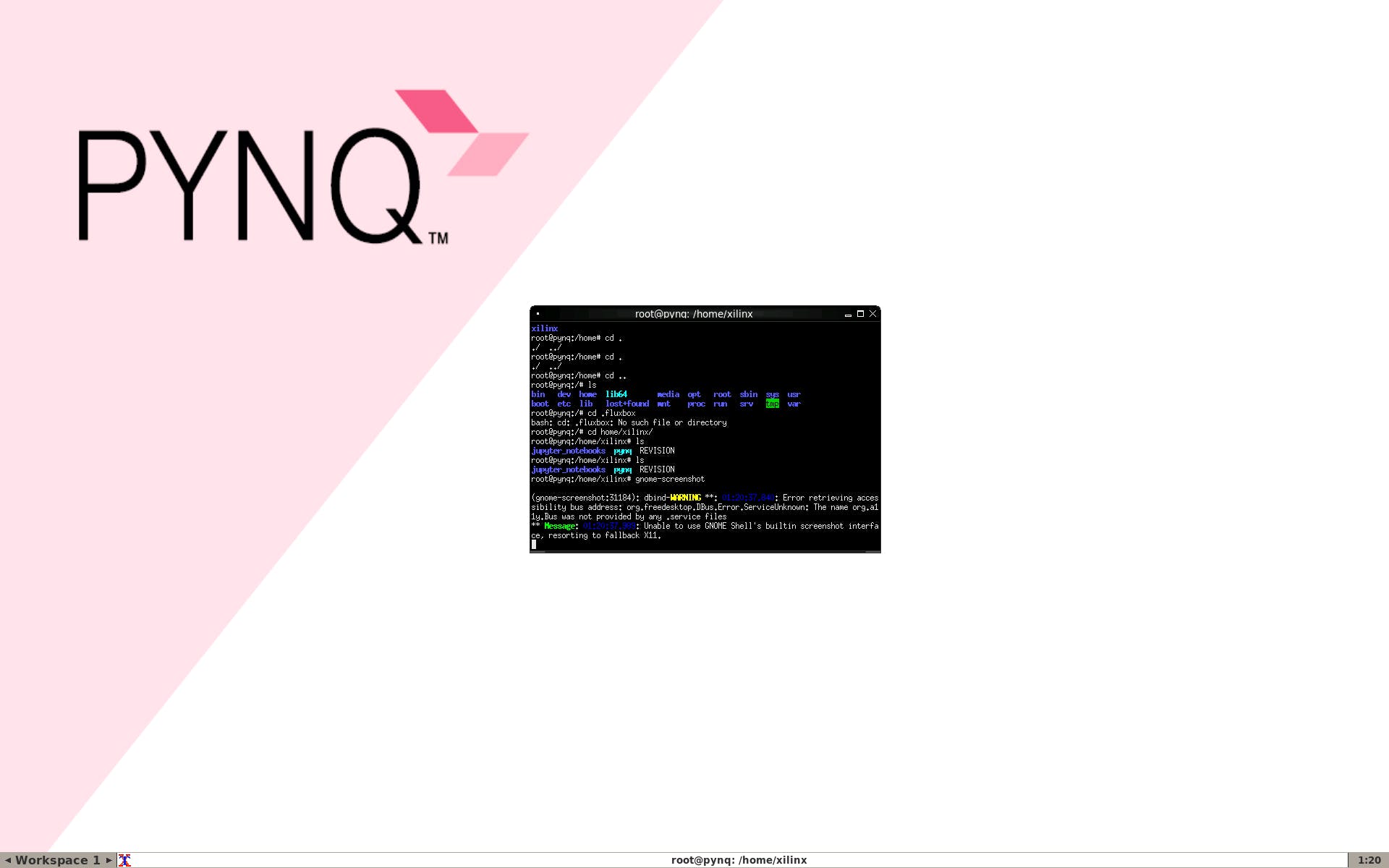
启动后，我们首先必须通过删除损坏的存储库来修复一些错误。

sudo rm -r /var/lib/apt/lists/*

这使我们可以根据需要安装所有软件包以使用该平台。

第 2 步：安装 Movidius NCSDK

因此，为了让 AI 和计算机视觉发挥作用，我们可以利用 Movidius NCS 来运行我们的项目。Ultra96 没有演练，所以我们基本上通过 https://movidius.github.io/blog/ncs-apps-on-rpi/ 引用了这个

首先我们必须安装依赖项，这部分不附带 PYNQ，所以我们将安装它们以确保一切正常。

apt-get install libgstreamer1.0-0 gstreamer1.0-plugins-base gstreamer1.0-plugins-good gstreamer1.0-plugins-bad gstreamer1.0-plugins-ugly gstreamer1.0-libav gstreamer1.0-doc gstreamer1.0-tools libgstreamer-plugins-base1.0-dev
apt-get install libgtk-3-dev
apt-get install -y libprotobuf-dev libleveldb-dev libsnappy-dev
apt-get install -y  libopencv-dev libhdf5-serial-dev 
apt-get install -y protobuf-compiler byacc libgflags-dev 
apt-get install -y libgoogle-glog-dev liblmdb-dev libxslt-dev 

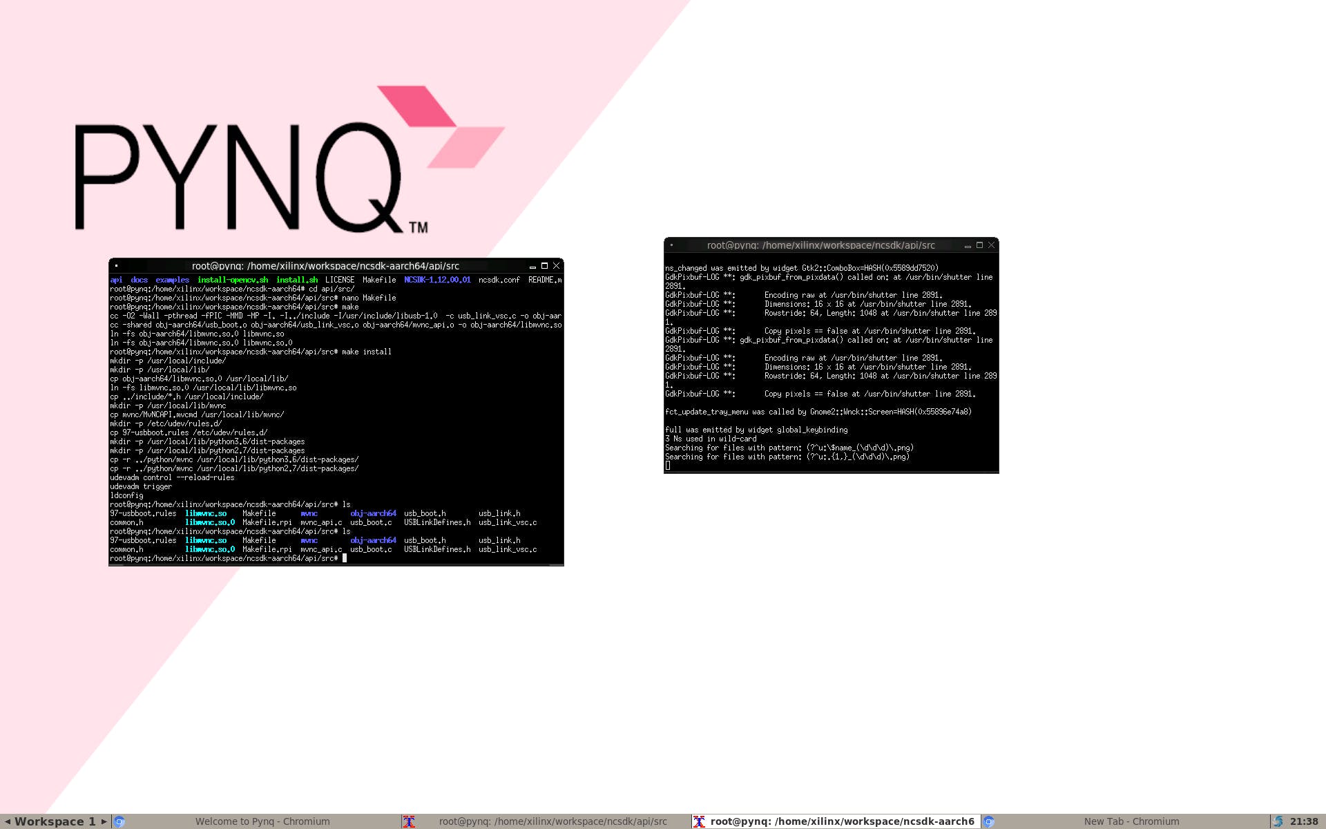
接下来我们可以安装 NCSDK SDK，它包含可以将应用程序连接到 NCS 的 API。由于 NCSDK 不是为 Ultra96 构建的，我们可以对markjay4k版本的解决方法进行以下修改

cd /home/xilinx/
mkdir -p workspace
cd workspace
git clone https://github.com/markjay4k/ncsdk-aarch64.git
cd ncsdk/api/src
make
make install

这个解决方法应该让我们使用 Ultra96 和 PYNQ 的 NCSDK API

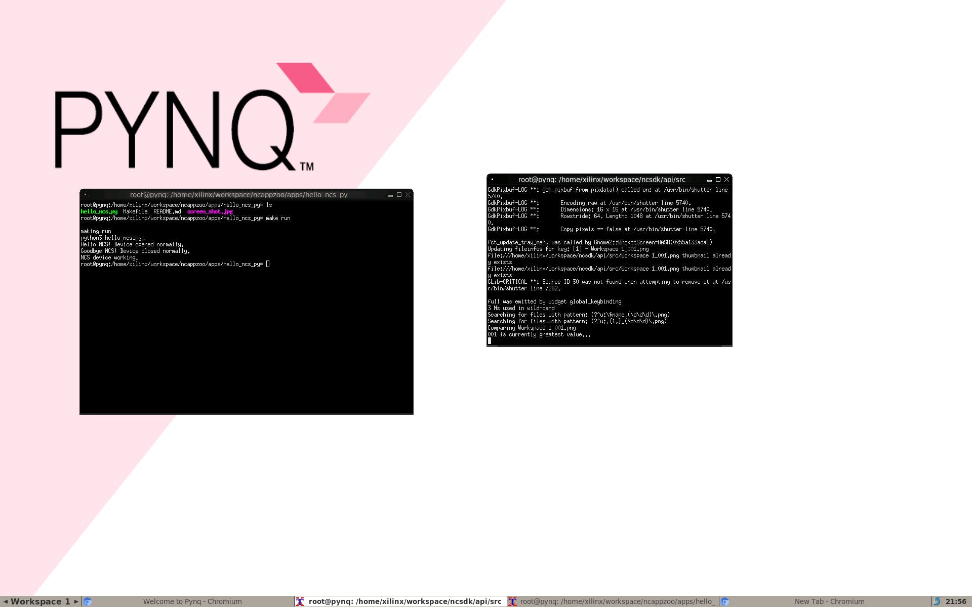
接下来我们将尝试让 NcAppZoo 和 Hello World 为 Neural Computing Stick 运行，我们需要在 pynq 上重复旧的 python 3.6

cd /home/xilinx/workspace
git clone https://github.com/movidius/ncappzoo
cd ncappzoo/apps/hello_ncs_py
make run

你刚刚让 NCS 在 aarch64 上运行 :)

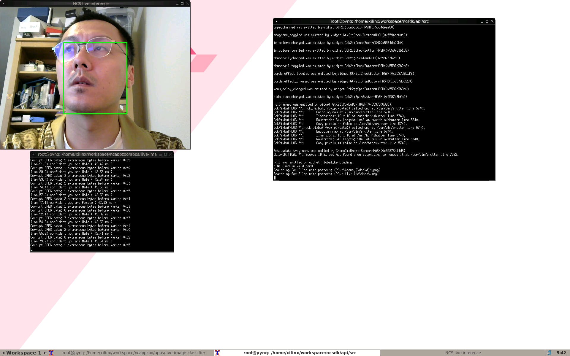
第 3 步：使用 Ultra96 和 NCS 实现边缘人工智能

我们可以通过多种方式制作触发器，因为这是一个基于 AI 的应用程序，我将制作一个基于 AI 的触发器。在本指南中，我们将使用经过预训练并使用 Caffe 的 SSD 神经网络，检测结果将是垃圾。因此，我们还将学习如何通过一些工作来利用其他神经网络。

在这一步中，我们之前已经训练了通过 caffe 模型，我们必须在另一台机器上编译图形，因为我们只安装了 API 而不是工具包，因为它们不是为 aarch64 构建的。然而，由于 API 有效，我们可以简单地在另一台机器上构建它并将图形文件传输到 Ultra96。FPGA 可以处理所有的 CV2，这里的 Movidius NCS 将运行推理以进行对象检测和图像分类，如下图所示，我们将通过在这里进行实时图像分类来确定基础。

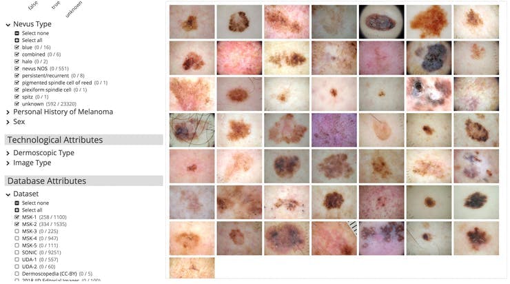
第 4 步：收集皮肤癌的图像数据集

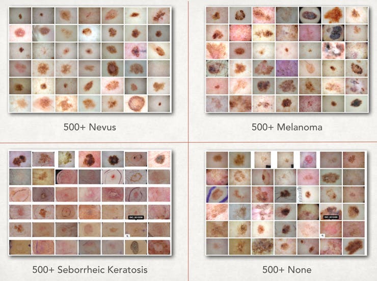
我们首先需要皮肤癌数据集，虽然有很多地方可以获取，但 isic-archive 成为最简单的一个。对于这部分，我们只需要大约 500 张痣、黑色素瘤和脂溢性角化病之间的图像，以及 500 张其他任何东西的随机图像。为了获得更高的准确性，我们必须使用更多的数据，这只是为了开始训练。获取数据的最简单方法是通过下面的图片使用 https://isic-archive.com/#images

之后，我们可以将图像标记到一个文件夹中，并将它们命名为 nevus-00.jpg、melanoma-00.jpg 以便我们可以轻松地构建我们的 lmdb。

第 5 步：设置训练服务器

机器学习训练使用了大量的处理能力，因此它们通常成本很高。在本文中，我们将重点介绍面向英特尔 AI Academy成员免费提供的 AI DevCloud。

为了构建皮肤癌 AI，我们使用 Caffe 框架，主要是因为英特尔 Movidius NCS 的 AI on the Edge 支持。Caffe 是由伯克利视觉与学习中心 (BVLC) 开发的深度学习框架，使用 caffe 框架训练我们的算法模型有 4 个步骤。这样，Xilinx 的 FPGA 可以专注于 openCV，NCS 可以专注于推理。

• 数据准备，我们清理图像并将它们存储到 LMDB。
• 模型定义 prototxt 文件，定义参数并选择 CNN 架构。
• Solver Definition prototxt 文件，定义模型优化的求解器参数
• 模型训练，我们执行caffe命令得到我们的.caffemodel算法文件

在 Devcloud 上，我们可以检查这些是否可用，只需转到

cd /glob/deep-learning/py-faster-rcnn/caffe-fast-rcnn/build/tools

第 6 步：准备 LMDB 进行训练

一旦我们设置好 DevCloud，我们就可以构建它

mkdir skincancerai
cd skincancerai
mkdir input
cd input
mkdir train 

从那里我们可以将我们之前设置的所有数据放入文件夹中

scp ./* colfax:/home/[youruser_name]/skincancerai/input/train/

之后，我们可以通过这种方式构建我们的 lmdb。我们通过以下几组来做到这一点

• 数据集的 5/6 将用于训练，1/6 用于验证，因此我们可以计算模型的准确性
• 我们将所有图像的大小调整为 227x227，以遵循与 BVLC 相同的标准
• 直方图均衡化应用于所有训练图像以调整对比度。
• 并将它们存储在 train_lmdb 和 validation_lmdb 中
• 使用 make_datum 标记 lmdb 内的所有图像数据集

import os
import glob
import random
import numpy as np
import cv2
import caffe
from caffe.proto import caffe_pb2
import lmdb
#We use 227x227 from BVLC
IMAGE_WIDTH = 227
IMAGE_HEIGHT = 227
def transform_img(img, img_width=IMAGE_WIDTH, img_height=IMAGE_HEIGHT):
  img[:, :, 0] = cv2.equalizeHist(img[:, :, 0])
  img[:, :, 1] = cv2.equalizeHist(img[:, :, 1])
  img[:, :, 2] = cv2.equalizeHist(img[:, :, 2])
  img = cv2.resize(img, (img_width, img_height), interpolation = cv2.INTER_CUBIC)
  return img
def make_datum(img, label):
  return caffe_pb2.Datum(
      channels=3,
      width=IMAGE_WIDTH,
      height=IMAGE_HEIGHT,
      label=label,
      data=np.rollaxis(img, 2).tostring())
train_lmdb = '/home/[your_username]/skincancerai/input/train_lmdb'
validation_lmdb = '/home/[youser_username]/skincancerai/input/validation_lmdb'
os.system('rm -rf  ' + train_lmdb)
os.system('rm -rf  ' + validation_lmdb)
train_data = [img for img in glob.glob("./input/train/*jpg")]
random.shuffle(train_data)
print 'Creating train_lmdb'
in_db = lmdb.open(train_lmdb, map_size=int(1e12))
with in_db.begin(write=True) as in_txn:
  for in_idx, img_path in enumerate(train_data):
      if in_idx %  6 == 0:
          continue
      img = cv2.imread(img_path, cv2.IMREAD_COLOR)
      img = transform_img(img, img_width=IMAGE_WIDTH, img_height=IMAGE_HEIGHT)
      if 'none' in img_path:
          label = 0
      elif 'nevus' in img_path:
          label = 1
      elif 'melanoma' in img_path:
          label = 2
      else:
          label = 3
      datum = make_datum(img, label)
      in_txn.put('{:0>5d}'.format(in_idx), datum.SerializeToString())
      print '{:0>5d}'.format(in_idx) + ':' + img_path
in_db.close()
print '\nCreating validation_lmdb'
in_db = lmdb.open(validation_lmdb, map_size=int(1e12))
with in_db.begin(write=True) as in_txn:
  for in_idx, img_path in enumerate(train_data):
      if in_idx % 6 != 0:
          continue
      img = cv2.imread(img_path, cv2.IMREAD_COLOR)
      img = transform_img(img, img_width=IMAGE_WIDTH, img_height=IMAGE_HEIGHT)
      if 'none' in img_path:
          label = 0
      elif 'nevus' in img_path:
          label = 1
      elif 'melanoma' in img_path:
          label = 2
      else:
          label = 3
      datum = make_datum(img, label)
      in_txn.put('{:0>5d}'.format(in_idx), datum.SerializeToString())
      print '{:0>5d}'.format(in_idx) + ':' + img_path
in_db.close()
print '\nFinished processing all images'

之后我们将运行脚本

python2 create_lmdb.py

获取所有 LMDB。完成后，我们需要获取训练数据的平均图像。作为 caffe 的一部分，我们可以通过

cd /glob/deep-learning/py-faster-rcnn/caffe-fast-rcnn/build/toolscompute_image_mean -backend=lmdb /home/[your_user]/skincancerai/input/train_lmdb /home/[your_user]/skincancerai/input/mean.binaryproto

上面的命令将生成训练数据的平均图像。每个输入图像将减去平均图像，使每个特征像素的均值为零。这是监督机器学习预处理中常用的方法。

第 7 步：设置模型定义和求解器定义

我们现在需要设置模型定义和求解器定义，在本文中我们将使用 bvlc_reference_net，可以在https://github.com/BVLC/caffe/tree/master/models/bvlc_reference_caffenet看到

下面是 train.prototxt 的修改版本

name: "CaffeNet"
layer {
name: "data"
type: "Data"
top: "data"
top: "label"
include {
  phase: TRAIN
}
transform_param {
  mirror: true
  crop_size: 227
  mean_file: "/home/[your_username]/skincancerai/input/mean.binaryproto"
}
data_param {
  source: "/home/[your_username]/skincancerai/input/train_lmdb"
  batch_size: 128
  backend: LMDB
}
}
layer {
name: "data"
type: "Data"
top: "data"
top: "label"
include {
  phase: TEST
}
transform_param {
  mirror: false
  crop_size: 227
  mean_file: "/home/[your_username]/skincancerai/input/mean.binaryproto"
}
# mean pixel / channel-wise mean instead of mean image
#  transform_param {
#    crop_size: 227
#    mean_value: 104
#    mean_value: 117
#    mean_value: 123
#    mirror: true
#  }
data_param {
  source: "/home/[your_username]/skincancerai/input/validation_lmdb"
  batch_size: 36
  backend: LMDB
}
}
layer {
name: "conv1"
type: "Convolution"
bottom: "data"
top: "conv1"
param {
  lr_mult: 1
  decay_mult: 1
}
param {
  lr_mult: 2
  decay_mult: 0
}
convolution_param {
  num_output: 96
  kernel_size: 11
  stride: 4
  weight_filler {
    type: "gaussian"
    std: 0.01
  }
  bias_filler {
    type: "constant"
    value: 0
  }
}
}
layer {
name: "relu1"
type: "ReLU"
bottom: "conv1"
top: "conv1"
}
layer {
name: "pool1"
type: "Pooling"
bottom: "conv1"
top: "pool1"
pooling_param {
  pool: MAX
  kernel_size: 3
  stride: 2
}
}
layer {
name: "norm1"
type: "LRN"
bottom: "pool1"
top: "norm1"
lrn_param {
  local_size: 5
  alpha: 0.0001
  beta: 0.75
}
}
layer {
name: "conv2"
type: "Convolution"
bottom: "norm1"
top: "conv2"
param {
  lr_mult: 1
  decay_mult: 1
}
param {
  lr_mult: 2
  decay_mult: 0
}
convolution_param {
  num_output: 256
  pad: 2
  kernel_size: 5
  group: 2
  weight_filler {
    type: "gaussian"
    std: 0.01
  }
  bias_filler {
    type: "constant"
    value: 1
  }
}
}
layer {
name: "relu2"
type: "ReLU"
bottom: "conv2"
top: "conv2"
}
layer {
name: "pool2"
type: "Pooling"
bottom: "conv2"
top: "pool2"
pooling_param {
  pool: MAX
  kernel_size: 3
  stride: 2
}
}
layer {
name: "norm2"
type: "LRN"
bottom: "pool2"
top: "norm2"
lrn_param {
  local_size: 5
  alpha: 0.0001
  beta: 0.75
}
}
layer {
name: "conv3"
type: "Convolution"
bottom: "norm2"
top: "conv3"
param {
  lr_mult: 1
  decay_mult: 1
}
param {
  lr_mult: 2
  decay_mult: 0
}
convolution_param {
  num_output: 384
  pad: 1
  kernel_size: 3
  weight_filler {
    type: "gaussian"
    std: 0.01
  }
  bias_filler {
    type: "constant"
    value: 0
  }
}
}
layer {
name: "relu3"
type: "ReLU"
bottom: "conv3"
top: "conv3"
}
layer {
name: "conv4"
type: "Convolution"
bottom: "conv3"
top: "conv4"
param {
  lr_mult: 1
  decay_mult: 1
}
param {
  lr_mult: 2
  decay_mult: 0
}
convolution_param {
  num_output: 384
  pad: 1
  kernel_size: 3
  group: 2
  weight_filler {
    type: "gaussian"
    std: 0.01
  }
  bias_filler {
    type: "constant"
    value: 1
  }
}
}
layer {
name: "relu4"
type: "ReLU"
bottom: "conv4"
top: "conv4"
}
layer {
name: "conv5"
type: "Convolution"
bottom: "conv4"
top: "conv5"
param {
  lr_mult: 1
  decay_mult: 1
}
param {
  lr_mult: 2
  decay_mult: 0
}
convolution_param {
  num_output: 256
  pad: 1
  kernel_size: 3
  group: 2
  weight_filler {
    type: "gaussian"
    std: 0.01
  }
  bias_filler {
    type: "constant"
    value: 1
  }
}
}
layer {
name: "relu5"
type: "ReLU"
bottom: "conv5"
top: "conv5"
}
layer {
name: "pool5"
type: "Pooling"
bottom: "conv5"
top: "pool5"
pooling_param {
  pool: MAX
  kernel_size: 3
  stride: 2
}
}
layer {
name: "fc6"
type: "InnerProduct"
bottom: "pool5"
top: "fc6"
param {
  lr_mult: 1
  decay_mult: 1
}
param {
  lr_mult: 2
  decay_mult: 0
}
inner_product_param {
  num_output: 4096
  weight_filler {
    type: "gaussian"
    std: 0.005
  }
  bias_filler {
    type: "constant"
    value: 1
  }
}
}
layer {
name: "relu6"
type: "ReLU"
bottom: "fc6"
top: "fc6"
}
layer {
name: "drop6"
type: "Dropout"
bottom: "fc6"
top: "fc6"
dropout_param {
  dropout_ratio: 0.5
}
}
layer {
name: "fc7"
type: "InnerProduct"
bottom: "fc6"
top: "fc7"
param {
  lr_mult: 1
  decay_mult: 1
}
param {
  lr_mult: 2
  decay_mult: 0
}
inner_product_param {
  num_output: 4096
  weight_filler {
    type: "gaussian"
    std: 0.005
  }
  bias_filler {
    type: "constant"
    value: 1
  }
}
}
layer {
name: "relu7"
type: "ReLU"
bottom: "fc7"
top: "fc7"
}
layer {
name: "drop7"
type: "Dropout"
bottom: "fc7"
top: "fc7"
dropout_param {
  dropout_ratio: 0.5
}
}
layer {
name: "fc8"
type: "InnerProduct"
bottom: "fc7"
top: "fc8"
param {
  lr_mult: 1
  decay_mult: 1
}
param {
  lr_mult: 2
  decay_mult: 0
}
inner_product_param {
  num_output: 4
  weight_filler {
    type: "gaussian"
    std: 0.01
  }
  bias_filler {
    type: "constant"
    value: 0
  }
}
}
layer {
name: "accuracy"
type: "Accuracy"
bottom: "fc8"
bottom: "label"
top: "accuracy"
include {
  phase: TEST
}
}
layer {
name: "loss"
type: "SoftmaxWithLoss"
bottom: "fc8"
bottom: "label"
top: "loss"
} 

同时我们可以创建基于 train.prototxt 构建的 deploy.prototxt。这可以从 github repo 中看到。我们还将像创建 lmdb 文件一样创建 label.txt 文件

classes
None
Nevus
Melanoma 
Seborrheic Keratosis

之后我们需要solver.prototxt中的Solver Definition，它用于优化训练模型。因为我们依赖CPU，所以我们需要对下面的求解器定义做一些修改。

net: "/home/[your_username]/skincancerai/model/train.prototxt"
test_iter: 50
test_interval: 50
base_lr: 0.001
lr_policy: "step"
gamma: 0.1
stepsize: 50
display: 50
max_iter: 5000
momentum: 0.9
weight_decay: 0.0005
snapshot: 1000
snapshot_prefix: "/home/[your_username]/skincancerai/model"
solver_mode: CPU 

因为我们在这里处理的数据量很小，所以我们可以缩短测试迭代并尽可能快地获得我们的模型。简而言之，求解器将使用验证集每 50 次迭代计算模型的准确性。由于我们没有大量数据，求解器优化过程将每 1000 次迭代拍摄一次快照，最多运行 5000 次迭代。lr_policy: "step", stepsize: 2500, base_lr: 0.001 and gamma: 0.1 的当前配置是相当标准的，因为我们也可以通过bvlc 求解器文档尝试使用其他配置。

第 8 步：训练模型

由于我们使用的是免费的 AI DevCloud 并且一切就绪，我们可以使用Intel Caffe ，它使用安装在集群上的 Intel CPU 进行了优化。由于这是一个集群，我们可以使用以下命令简单地开始训练。

cd /glob/deep-learning/py-faster-rcnn/caffe-fast-rcnn/build/toolsecho caffe train --solver ~/skincancerai/model/solver.prototxt | qsub -o ~/skincancerai/model/output.txt -e ~/skincancerai/model/train.log

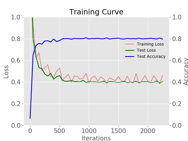
训练后的模型将是model_iter_1000.caffemodel、model_iter_2000.caffemodel等。使用 ISIC 提供的数据，您应该获得大约 70% 到 80% 的准确度。您可以通过以下命令绘制自己的曲线，

cd ~/skincancerai python2 plot_learning_curve.py ./model/train.log ./model/train.png

第 9 步：在具有 NCS 的 Ultra96 上部署和运行

在本文中，我们使用 Ultra96，这样我们就可以拥有一个可以随身携带的离线设备。我们已经在步骤 3 上运行了示例。由于我们在 aarch64 上没有激活工具包，我们可以在另一台机器上运行编译，然后将其复制到 ultra96

mvNCCompile deploy.prototxt -w 
model_iter_1000.caffemodel,model_iter_2000.caffemodel

这将为您提供图形文件，复制图形文件和标签文件并将其与我们修改的以下代码一起放在 CancerNet 下，将其复制到 Ultra96。我们现在有一个可以在家中使用的皮肤癌检测设备。我们可以在CancerNet下使用图形文件和categories.txt文件部署以下代码

#!/usr/bin/python3
# ****************************************************************************
# Copyright(c) 2017 Intel Corporation. 
# License: MIT See LICENSE file in root directory.
# ****************************************************************************
# Perform inference on a LIVE camera feed using DNNs on 
# Intel® Movidius™ Neural Compute Stick (NCS)
import os
import cv2
import sys
import numpy
import ntpath
import argparse
import mvnc.mvncapi as mvnc
# Variable to store commandline arguments
ARGS                 = None
# OpenCV object for video capture
camera               = None
# ---- Step 1: Open the enumerated device and get a handle to it -------------
def open_ncs_device():
   # Look for enumerated NCS device(s); quit program if none found.
   devices = mvnc.EnumerateDevices()
   if len( devices ) == 0:
       print( "No devices found" )
       quit()
   # Get a handle to the first enumerated device and open it
   device = mvnc.Device( devices[0] )
   device.OpenDevice()
   return device
# ---- Step 2: Load a graph file onto the NCS device -------------------------
def load_graph( device ):
   # Read the graph file into a buffer
   with open( ARGS.graph, mode='rb' ) as f:
       blob = f.read()
   # Load the graph buffer into the NCS
   graph = device.AllocateGraph( blob )
   return graph
# ---- Step 3: Pre-process the images ----------------------------------------
def pre_process_image( frame ):
   # Resize image [Image size is defined by choosen network, during training]
   img = cv2.resize( frame, tuple( ARGS.dim ) )
   # Extract/crop a section of the frame and resize it
   height, width, channels = frame.shape
   x1 = int( width / 3 )
   y1 = int( height / 4 )
   x2 = int( width * 2 / 3 )
   y2 = int( height * 3 / 4 )
   cv2.rectangle( frame, ( x1, y1 ) , ( x2, y2 ), ( 0, 255, 0 ), 2 )
   img = frame[ y1 : y2, x1 : x2 ]
   # Resize image [Image size if defined by choosen network, during training]
   img = cv2.resize( img, tuple( ARGS.dim ) )
   # Convert BGR to RGB [OpenCV reads image in BGR, some networks may need RGB]
   if( ARGS.colormode == "rgb" ):
       img = img[:, :, ::-1]
   # Mean subtraction & scaling [A common technique used to center the data]
   img = img.astype( numpy.float16 )
   img = ( img - numpy.float16( ARGS.mean ) ) * ARGS.scale
   return img
# ---- Step 4: Read & print inference results from the NCS -------------------
def infer_image( graph, img, frame ):
   # Load the image as a half-precision floating point array
   graph.LoadTensor( img, 'user object' )
   # Get the results from NCS
   output, userobj = graph.GetResult()
   # Find the index of highest confidence 
   top_prediction = output.argmax()
   # Get execution time
   inference_time = graph.GetGraphOption( mvnc.GraphOption.TIME_TAKEN )
   print(  "I am %3.1f%%" % (100.0 * output[top_prediction] ) + " confidant"
           + " it is " + labels[top_prediction]
           + " ( %.2f ms )" % ( numpy.sum( inference_time ) ) )
   displaystring = str(100.0 * output[top_prediction]) + " " + labels[top_prediction]
   # If a display is available, show the image on which inference was performed
   if 'DISPLAY' in os.environ:
       textsize = cv2.getTextSize(displaystring, cv2.FONT_HERSHEY_SIMPLEX, 1, 2)[0]
       textX = (frame.shape[1] - textsize[0])/2
       cv2.putText(frame, displaystring, (int(textX),450), cv2.FONT_HERSHEY_SIMPLEX, 1, (255,0,0),2)
       cv2.imshow( 'Skin Cancer AI', frame )
# ---- Step 5: Unload the graph and close the device -------------------------
def close_ncs_device( device, graph ):
   graph.DeallocateGraph()
   device.CloseDevice()
   camera.release()
   cv2.destroyAllWindows()
# ---- Main function (entry point for this script ) --------------------------
def main():
   device = open_ncs_device()
   graph = load_graph( device )
   # Main loop: Capture live stream & send frames to NCS
   while( True ):
       ret, frame = camera.read()
       img = pre_process_image( frame )
       infer_image( graph, img, frame )
       # Display the frame for 5ms, and close the window so that the next
       # frame can be displayed. Close the window if 'q' or 'Q' is pressed.
       if( cv2.waitKey( 5 ) & 0xFF == ord( 'q' ) ):
           break
   close_ncs_device( device, graph )
# ---- Define 'main' function as the entry point for this script -------------
if __name__ == '__main__':
   parser = argparse.ArgumentParser(
                        description="Image classifier using \
                        Intel® Movidius™ Neural Compute Stick." )
   parser.add_argument( '-g', '--graph', type=str,
                        default='CancerNet/graph',
                        help="Absolute path to the neural network graph file." )
   parser.add_argument( '-v', '--video', type=int,
                        default=0,
                        help="Index of your computer's V4L2 video device. \
                              ex. 0 for /dev/video0" )
   parser.add_argument( '-l', '--labels', type=str,
                        default='./CancerNet/categories.txt',
                        help="Absolute path to labels file." )
   parser.add_argument( '-M', '--mean', type=float,
                        nargs='+',
                        default=[78.42633776, 87.76891437, 114.89584775],
                        help="',' delimited floating point values for image mean." )
   parser.add_argument( '-S', '--scale', type=float,
                        default=1,
                        help="Absolute path to labels file." )
   parser.add_argument( '-D', '--dim', type=int,
                        nargs='+',
                        default=[227, 227],
                        help="Image dimensions. ex. -D 224 224" )
   parser.add_argument( '-c', '--colormode', type=str,
                        default="rgb",
                        help="RGB vs BGR color sequence. This is network dependent." )
   ARGS = parser.parse_args()
   # Create a VideoCapture object
   camera = cv2.VideoCapture( ARGS.video )
   # Set camera resolution
   camera.set( cv2.CAP_PROP_FRAME_WIDTH, 620 )
   camera.set( cv2.CAP_PROP_FRAME_HEIGHT, 480 )
   # Load the labels file
   labels =[ line.rstrip('\n') for line in
             open( ARGS.labels ) if line != 'classes\n']
   main()
# ==== End of file ===========================================================

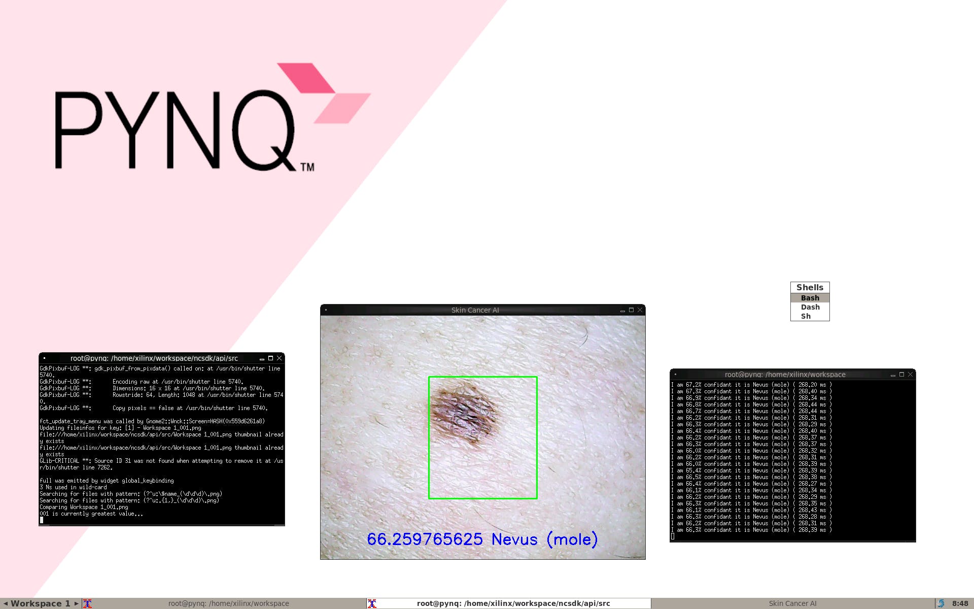
从这里开始，我们就有了皮肤癌 AI 分类，只需在文件夹中运行以下命令。

python3 live-image-classifier.py 

我们可以检测到我们自己的痣

当有黑色素瘤时

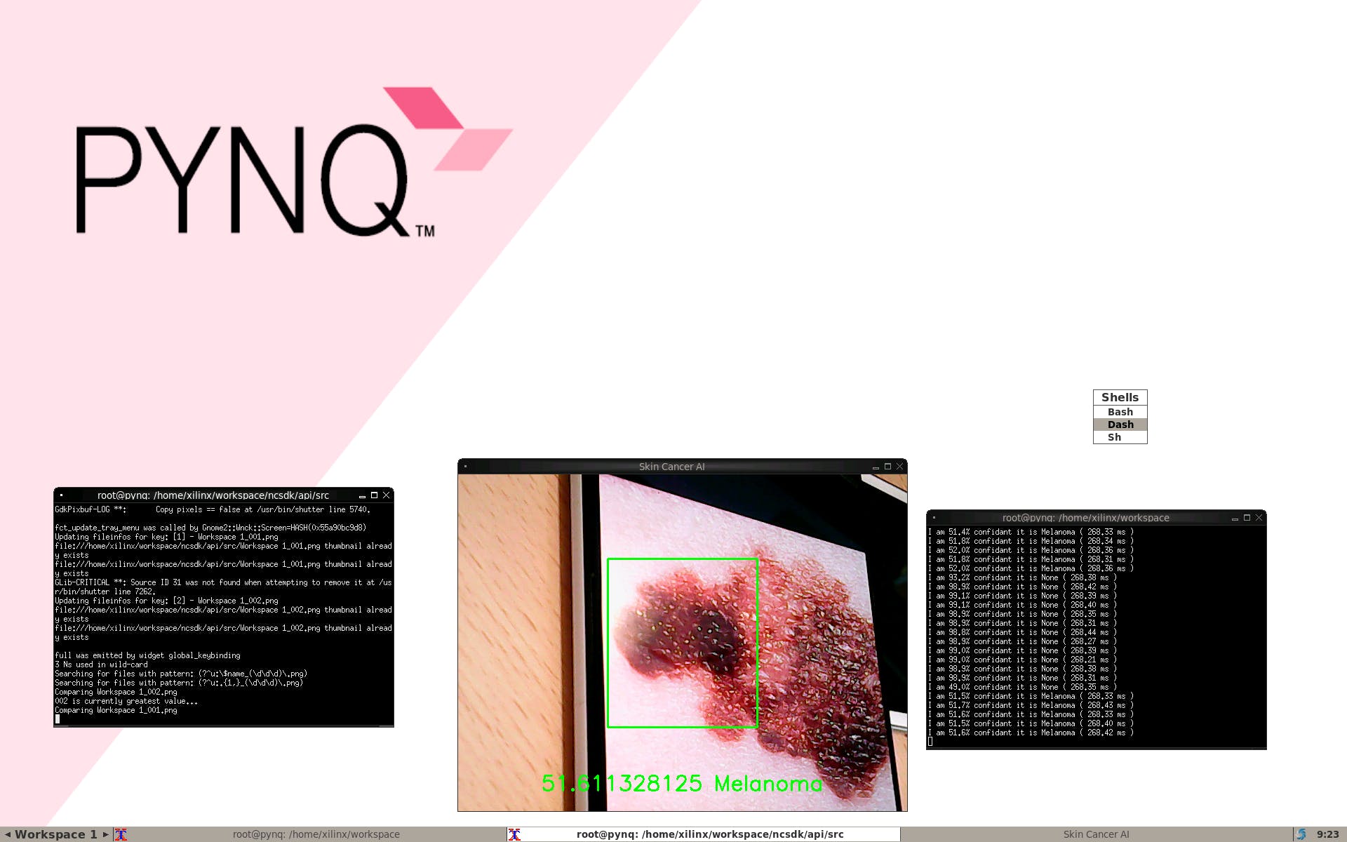
我们可以看到完整的演示